27 效率调优
Efficiency Tuning
本节译者:焦睿宇、苏田园
初次校审:张梓源
二次校审:邱怡轩(Claude Code+GLM 辅助)
This chapter provides a grab bag of techniques for optimizing Stan code, including vectorization, sufficient statistics, and conjugacy. At a coarse level, efficiency involves both the amount of time required for a computation and the amount of memory required. For practical applied statistical modeling, we are mainly concerned with reducing wall time (how long a program takes as measured by a clock on the wall) and keeping memory requirements within available bounds.
本章提供了一系列优化 Stan 代码的技术,包括向量化、充分统计量和共轭性。粗略地讲,效率包括计算所需的时间和内存需求。对于实际应用的统计建模,我们主要关注减少墙上时间(用墙上时钟测量的程序执行时间),并将内存需求保持在可用范围内。
27.1 What is efficiency?
什么是效率?
The standard algorithm analyses in computer science measure efficiency asymptotically as a function of problem size (such as data, number of parameters, etc.) and typically do not consider constant additive factors like startup times or multiplicative factors like speed of operations. In practice, the constant factors are important; if run time can be cut in half or more, that’s a huge gain. This chapter focuses on both the constant factors involved in efficiency (such as using built-in matrix operations as opposed to naive loops) and on asymptotic efficiency factors (such as using linear algorithms instead of quadratic algorithms in loops).
计算机科学中的标准算法分析将效率渐近地测量为问题规模(如数据、参数数量等)的函数,通常不考虑启动时间等常数加法因子或运算速度等常数乘法因子。在实践中,常数因子很重要;如果运行时间可以减少一半或更多,那将是一个巨大的收益。本章重点关注效率中涉及的常数因子(例如使用内置矩阵运算而非简单的循环)和渐近效率因子(例如在循环中使用线性算法而非二次算法)。
27.2 Efficiency for probabilistic models and algorithms
概率模型和算法的效率
Stan programs express models which are intrinsically statistical in nature. The algorithms applied to these models may or may not themselves be probabilistic. For example, given an initial value for parameters (which may itself be given deterministically or generated randomly), Stan’s optimization algorithm (L-BFGS) for penalized maximum likelihood estimation is purely deterministic. Stan’s sampling algorithms are based on Markov chain Monte Carlo algorithms, which are probabilistic by nature at every step. Stan’s variational inference algorithm (ADVI) is probabilistic despite being an optimization algorithm; the randomization lies in a nested Monte Carlo calculation for an expected gradient.
Stan 程序所表达的模型本质上是统计性的。应用于这些模型的算法本身可能是概率性的,也可能不是。例如,给定参数的初始值(其本身可以是确定性的或随机生成的),用于惩罚最大似然估计的 Stan 优化算法(L-BFGS)是纯确定性的。Stan 的采样算法基于马尔可夫链蒙特卡罗(Markov Chain Monte Carlo, MCMC)算法,该算法在每一步都具有概率性。Stan 的变分推断算法(ADVI)虽然是一种优化算法,但却是概率性的,其随机化在于对期望梯度的嵌套蒙特卡罗计算。
With probabilistic algorithms, there will be variation in run times (and maybe memory usage) based on the randomization involved. For example, by starting too far out in the tail, iterative algorithms underneath the hood, such as the solvers for ordinary differential equations, may take different numbers of steps. Ideally this variation will be limited; when there is a lot of variation it can be a sign that there is a problem with the model’s parameterization in a Stan program or with initialization.
对于概率性算法,由于涉及随机化,运行时间(可能还有内存使用)会有所变化。例如,由于从分布尾部过远处开始,底层的迭代算法(如常微分方程求解器)可能需要不同数量的步骤。理想情况下,这种变化是有限的;当有较大变化时,这可能意味着 Stan 程序中模型的参数化或初始化出现问题。
A well-behaved Stan program will have low variance between runs with different random initializations and differently seeded random number generators. But sometimes an algorithm can get stuck in one part of the posterior, typically due to high curvature. Such sticking almost always indicates the need to reparameterize the model. Just throwing away Markov chains with apparently poor behavior (slow, or stuck) can lead to bias in posterior estimates. This problem with getting stuck can often be overcome by lowering the initial step size to avoid getting stuck during adaptation and increasing the target acceptance rate in order to target a lower step size. This is because smaller step sizes allow Stan’s gradient-based algorithms to better follow the curvature in the density or penalized maximum likelihood being fit.
一个表现良好的 Stan 程序在不同随机初始化和不同随机数种子下的运行结果具有较低的方差。但有时算法可能会陷入后验分布的某个区域,通常是由于高曲率造成的。这种停滞几乎总是表明需要对模型进行重参数化。仅仅丢弃具有明显不良行为(缓慢或停滞)的马尔可夫链可能导致后验估计的偏差。这种陷入停滞的问题通常可以通过降低初始步长来克服,以避免在自适应过程中陷入困境,并增加目标接受率以达到较低的步长。这是因为较小的步长允许 Stan 的基于梯度的算法更好地遵循密度中的曲率或被惩罚的最大似然。
27.3 Statistical vs. computational efficiency
统计效率与计算效率
There is a difference between pure computational efficiency and statistical efficiency for Stan programs fit with sampling-based algorithms. Computational efficiency measures the amount of time or memory required for a given step in a calculation, such as an evaluation of a log posterior or penalized likelihood.
对于使用基于采样算法的 Stan 程序,纯计算效率和统计效率之间存在差异。计算效率衡量计算中给定步骤所需的时间或内存量,例如对数后验或惩罚似然的评估。
Statistical efficiency typically involves requiring fewer steps in algorithms by making the statistical formulation of a model better behaved. The typical way to do this is by applying a change of variables (i.e., reparameterization) so that sampling algorithms mix better or optimization algorithms require less adaptation.
统计效率通常通过改善模型统计公式的表现来减少算法所需的步骤。实现这一点的典型方法是应用变量变换(即重参数化),以便采样算法更好地混合,或者优化算法需要更少的自适应。
27.4 Model conditioning and curvature
模型条件和曲率
Because Stan’s algorithms rely on step-based gradient-based approximations of the density (or penalized maximum likelihood) being fitted, posterior curvature not captured by this first-order approximation plays a central role in determining the statistical efficiency of Stan’s algorithms.
由于 Stan 的算法依赖于对所拟合的密度(或惩罚最大似然)的基于步长和梯度的近似,因此这种一阶近似没有捕捉到的后验曲率在决定 Stan 算法的统计效率方面起着核心作用。
A second-order approximation to curvature is provided by the Hessian, the matrix of second derivatives of the log density \(\log p(\theta)\) with respect to the parameter vector \(\theta\), defined as
曲率的二阶近似由 Hessian 提供,Hessian 是对数密度 \(\log p(\theta)\) 相对于参数向量 \(\theta\) 的二阶导数矩阵,定义为
\[ H(\theta) = \nabla \, \nabla \, \log p(\theta \mid y), \] so that
所以
\[ H_{i, j}(\theta) = \frac{\partial^2 \log p(\theta \mid y)} {\partial \theta_i \ \partial \theta_j}. \] For pure penalized maximum likelihood problems, the posterior log density \(\log p(\theta \mid y)\) is replaced by the penalized likelihood function \(\mathcal{L}(\theta) = \log p(y \mid \theta) - \lambda(\theta)\).
对于纯惩罚的最大似然问题,后验对数密度 \(\log p(\theta \mid y)\) 被惩罚似然函数 \(\mathcal{L}(\theta) = \log p(y \mid \theta) - \lambda(\theta)\) 取代。
Condition number and adaptation
条件数和自适应
A good gauge of how difficult a problem the curvature presents is given by the condition number of the Hessian matrix \(H\), which is the ratio of the largest to the smallest eigenvalue of \(H\) (assuming the Hessian is positive definite). This essentially measures the difference between the flattest direction of movement and the most curved. Typically, the step size of a gradient-based algorithm is bounded by the most sharply curved direction. With better conditioned log densities or penalized likelihood functions, it is easier for Stan’s adaptation, especially the diagonal adaptations that are used as defaults.
Hessian 矩阵 \(H\) 的条件数很好地衡量了曲率问题的难度,它是 \(H\) 最大特征值与最小特征值的比值(假设 Hessian 是正定的)。这本质上衡量了最平坦的方向与最弯曲的方向之间的差异。通常,基于梯度的算法的步长受到最陡峭弯曲方向的限制。具有条件更好的对数密度或惩罚似然函数时,Stan 的自适应更容易,尤其是用作默认值的对角自适应。
Unit scales without correlation
无相关性的单位尺度
Ideally, all parameters should be programmed so that they have unit scale and so that posterior correlation is reduced; together, these properties mean that there is no rotation or scaling required for optimal performance of Stan’s algorithms. For Hamiltonian Monte Carlo, this implies a unit mass matrix, which requires no adaptation as it is where the algorithm initializes.
理想情况下,所有参数都应该设置为具有单位尺度并减少后验相关性;这些性质意味着 Stan 算法的最佳性能不需要旋转或缩放。对于 Hamiltonian Monte Carlo(哈密顿蒙特卡罗),这意味着单位质量矩阵,由于这是算法初始化时使用的,因此不需要自适应。
Varying curvature
变曲率
In all but very simple models (such as multivariate normals), the Hessian will vary as \(\theta\) varies (an extreme example is Neal’s funnel, as naturally arises in hierarchical models with little or no data). The more the curvature varies, the harder it is for all of the algorithms with fixed adaptation parameters to find adaptations that cover the entire density well. Many of the variable transforms proposed are aimed at improving the conditioning of the Hessian and/or making it more consistent across the relevant portions of the density (or penalized maximum likelihood function) being fit.
在除非常简单的模型(如多元正态)外的所有模型中,Hessian 将随着 \(\theta\) 的变化而变化(一个极端的例子是 Neal 的漏斗分布,这在数据很少或没有数据的分层模型中自然出现)。曲率变化越大,具有固定自适应参数的算法就越难找到能覆盖整个密度的良好自适应。所提出的许多变量变换旨在改善 Hessian 的条件,和/或使其在所拟合的密度(或惩罚最大似然函数)的相关部分之间更加一致。
For all of Stan’s algorithms, the curvature along the path from the initial values of the parameters to the solution is relevant. For penalized maximum likelihood and variational inference, the solution of the iterative algorithm will be a single point, so this is all that matters. For sampling, the relevant “solution” is the typical set, which is the posterior volume where almost all draws from the posterior lies; thus, the typical set contains almost all of the posterior probability mass.
对于 Stan 的所有算法,从参数初始值到解的路径上的曲率是相关的。对于惩罚最大似然和变分推断,迭代算法的解将是一个点,所以这才是最重要的。对于采样,相关的“解”是典型集,即几乎所有后验抽样所在的后验区域;因此,典型集包含了几乎所有的后验概率质量。
With sampling, the curvature may vary dramatically between the points on the path from the initialization point to the typical set and within the typical set. This is why adaptation needs to run long enough to visit enough points in the typical set to get a good first-order estimate of the curvature within the typical set. If adaptation is not run long enough, sampling within the typical set after adaptation will not be efficient. We generally recommend at least one hundred iterations after the typical set is reached (and the first effective draw is ready to be realized). Whether adaptation has run long enough can be measured by comparing the adaptation parameters derived from a set of diffuse initial parameter values.
通过采样,曲率可以在从初始化点到典型集的路径上的点之间以及在典型集内显著变化。这就是为什么自适应需要运行足够长的时间来访问典型集中的足够多的点,以获得典型集中曲率的良好一阶估计。如果自适应运行的时间不够长,则在自适应之后在典型集内进行采样将是低效的。我们通常建议在达到典型集后至少进行一百次迭代(并且第一次有效抽样已准备好实现)。自适应是否已经运行足够长可以通过比较从一组扩散初始参数值导出的自适应参数来测量。
Reparameterizing with a change of variables
变量变换的重参数化
Improving statistical efficiency is achieved by reparameterizing the model so that the same result may be calculated using a density or penalized maximum likelihood that is better conditioned. Again, see the example of reparameterizing Neal’s funnel for an example, and also the examples in the change of variables chapter.
统计效率的提高可以通过对模型进行重参数化来实现,从而可以使用条件更好的密度或惩罚最大似然来计算相同的结果。具体可参阅重参数化 Neal 的漏斗分布的示例,以及变量变换章节中的示例。
One has to be careful in using change-of-variables reparameterizations when using maximum likelihood estimation, because they can change the result if the Jacobian term is inadvertently included in the revised likelihood model.
在使用最大似然估计时,必须小心使用变量变换重参数化,因为如果雅可比行列式项无意中包含在修正的似然模型中,可能会改变结果。
27.5 Well-specified models
设定良好的模型
Model misspecification, which roughly speaking means using a model that doesn’t match the data, can be a major source of slow code. This can be seen in cases where simulated data according to the model runs robustly and efficiently, whereas the real data for which it was intended runs slowly or may even have convergence and mixing issues. While some of the techniques recommended in the remaining sections of this chapter may mitigate the problem, the best remedy is a better model specification.
模型误设,大致是指使用一个与数据不匹配的模型,这可能是慢代码的主要来源。这体现在这样的情况中:根据模型模拟的数据运行稳健而高效,而其预期的真实数据运行缓慢,甚至可能出现收敛和混合的问题。虽然本章其余部分推荐的一些技术可以缓解这个问题,但最好的补救措施是更好的模型设定。
Counterintuitively, more complicated models often run faster than simpler models. One common pattern is with a group of parameters with a wide fixed prior such as normal(0, 1000)). This can fit slowly due to the mismatch between prior and posterior (the prior has support for values in the hundreds or even thousands, whereas the posterior may be concentrated near zero). In such cases, replacing the fixed prior with a hierarchical prior such as normal(mu, sigma), where mu and sigma are new parameters with their own hyperpriors, can be beneficial.
反直觉的是,更复杂的模型往往比更简单的模型运行更快。一个常见的模式是,一组参数有一个宽泛的固定先验,如 normal(0, 1000)。由于先验和后验的不匹配(先验对上百甚至上千的值有支持,而后验可能集中在零附近),这可能导致拟合缓慢。在这种情况下,用 normal(mu, sigma) 这样的分层先验代替固定先验可能会有好处,其中 mu 和 sigma 是有自己超先验的新参数。
27.6 Avoiding validation
避免验证
Stan validates all of its data structure constraints. For example, consider a transformed parameter defined to be a covariance matrix and then used as a covariance parameter in the model block.
Stan 验证了其所有的数据结构约束。例如,考虑一个被定义为协方差矩阵的转换参数,然后在模型块中作为协方差参数使用。
transformed parameters {
  cov_matrix[K] Sigma;
  // ...
}                               // first validation
model {
  y ~ multi_normal(mu, Sigma);  // second validation
  // ...
}
Because Sigma is declared to be a covariance matrix, it will be factored at the end of the transformed parameter block to ensure that it is positive definite. The multivariate normal log density function also validates that Sigma is positive definite. This test is expensive, having cubic run time (i.e., \(\mathcal{O}(N^3)\) for \(N \times N\) matrices), so it should not be done twice.
因为 Sigma 被声明为协方差矩阵,它将在转换参数块的末尾进行分解以确保它是正定的。多元正态对数密度函数也验证 Sigma 是正定的。这个测试很昂贵,具有三次方运行时间(即 \(N \times N\) 矩阵的 \(\mathcal{O}(N^3)\)),所以不应该做两次。
The test may be avoided by simply declaring Sigma to be a simple unconstrained matrix.
该测试可以通过简单地将 Sigma 声明为一个简单的无约束矩阵来避免。
transformed parameters {
  matrix[K, K] Sigma;
  // ...
}
model {
  y ~ multi_normal(mu, Sigma);  // only validation
}
Now the only validation is carried out by the multivariate normal.
现在,唯一的验证由多元正态函数执行。
27.7 Reparameterization
重参数化
Stan’s sampler can be slow in sampling from distributions with difficult posterior geometries. One way to speed up such models is through reparameterization. In some cases, reparameterization can dramatically increase effective sample size for the same number of iterations or even make programs that would not converge well behaved.
Stan 的采样器在从具有困难后验几何的分布中采样时可能很慢。加快此类模型的一种方法是通过重参数化。在某些情况下,重参数化可以在相同迭代次数下大幅增加有效样本量,甚至可以使原本不会收敛的程序表现良好。
Example: Neal’s funnel
例:Neal 的漏斗分布
In this section, we discuss a general transform from a centered to a non-centered parameterization (Papaspiliopoulos, Roberts, and Sköld 2007).1
在这一节中,我们将讨论从中心化到非中心参数化的一般转换 (Papaspiliopoulos, Roberts, and Sköld 2007)。2
This reparameterization is helpful when there is not much data, because it separates the hierarchical parameters and lower-level parameters in the prior.
在数据不多的情况下,这种重参数化很有帮助,因为它将先验中的高层参数和低层参数分开。
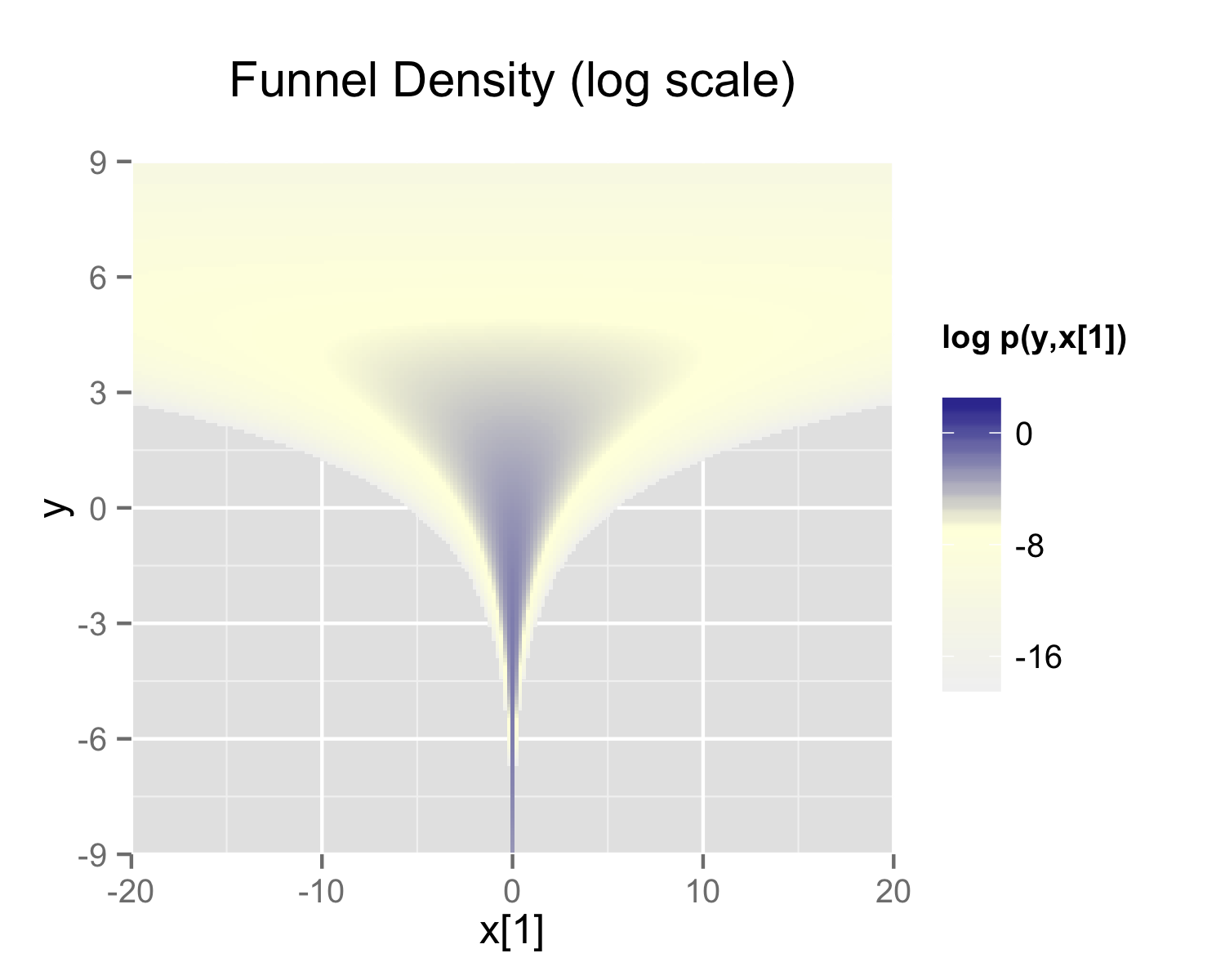
Neal (2003) defines a distribution that exemplifies the difficulties of sampling from some hierarchical models. Neal’s example is fairly extreme, but can be trivially reparameterized in such a way as to make sampling straightforward. Neal’s example has support for \(y \in \mathbb{R}\) and \(x \in \mathbb{R}^9\) with density
Neal (2003) 定义了一个分布,体现了从一些层次模型中取样的困难。Neal 的例子是相当极端的,但是可以以一种简单的方式重参数化,从而使抽样变得简单。Neal 的例子对 \(y \in \mathbb{R}\) 和 \(x \in \mathbb{R}^9\) 有支持,密度为
\[ p(y,x) = \textsf{normal}(y \mid 0,3) \times \prod_{n=1}^9 \textsf{normal}(x_n \mid 0,\exp(y/2)). \]
The probability contours are shaped like ten-dimensional funnels. The funnel’s neck is particularly sharp because of the exponential function applied to \(y\). A plot of the log marginal density of \(y\) and the first dimension \(x_1\) is shown in the following plot.
概率轮廓的形状像十维的漏斗。由于应用于 \(y\) 的指数函数,漏斗的颈部特别尖锐。下图是 \(y\) 的对数边际密度和第一维 \(x_1\) 的图。
The funnel can be implemented directly in Stan as follows.
漏斗可以直接在 Stan 中实现,具体方法如下。
parameters {
real y;
vector[9] x;
}
model {
y ~ normal(0, 3);
x ~ normal(0, exp(y/2));
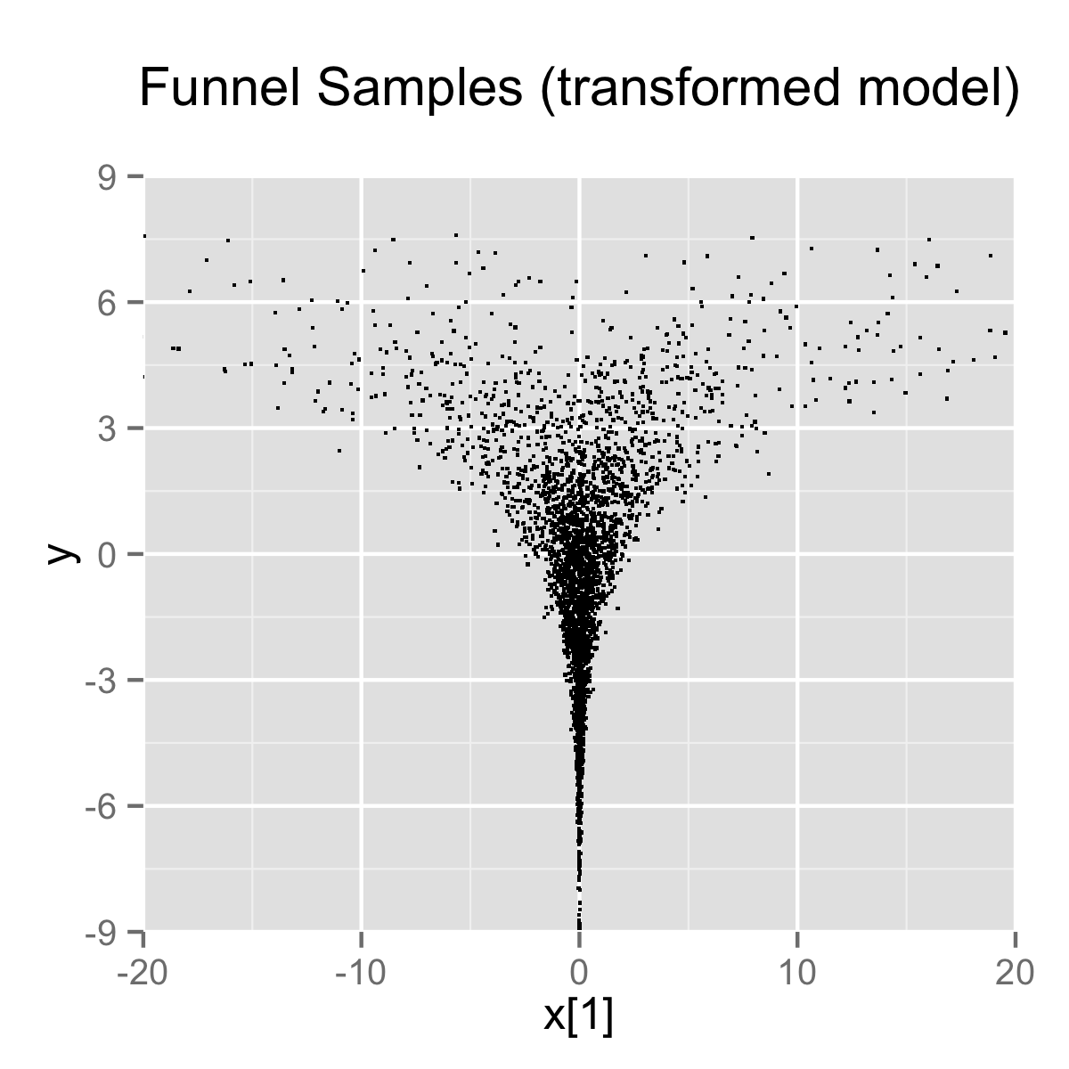
}When the model is expressed this way, Stan has trouble sampling from the neck of the funnel, where \(y\) is small and thus \(x\) is constrained to be near 0. This is due to the fact that the density’s scale changes with \(y\), so that a step size that works well in the body will be too large for the neck, and a step size that works in the neck will be inefficient in the body. This can be seen in the following plots.
当模型以这种方式表达时,Stan 很难从漏斗的颈部取样,因为那里的 \(y\) 很小,因此 \(x\) 被限制在0附近。这是由于密度的尺度随着 \(y\) 的变化而变化,因此在主体中效果好的步长对颈部来说会过大,而在颈部效果好的步长在主体中会效率低下。这可以从下面的图中看出。
In this particular instance, because the analytic form of the density is known, the model can be converted to the following more efficient form.
在这个特殊的例子中,由于密度函数的解析形式是已知的,因此模型可以转换为以下更有效的形式。
parameters {
  real y_raw;
  vector[9] x_raw;
}
transformed parameters {
  real y;
  vector[9] x;

  y = 3.0 * y_raw;
  x = exp(y/2) * x_raw;
}
model {
  y_raw ~ std_normal(); // implies y ~ normal(0, 3)
  x_raw ~ std_normal(); // implies x ~ normal(0, exp(y/2))
}
In this second model, the parameters x_raw and y_raw are sampled as independent standard normals, which is easy for Stan. These are then transformed into draws from the funnel. In this case, the same transform may be used to define Monte Carlo directly based on independent standard normal draws; Markov chain Monte Carlo methods are not necessary. If such a reparameterization were used in Stan code, it is useful to provide a comment indicating what the distribution for the parameter implies for the distribution of the transformed parameter.
在第二个模型中,参数 x_raw 和 y_raw 是按照独立标准正态分布采样的,这对 Stan 来说很容易。然后这些被转换为漏斗的采样样本。在这种情况下,同样的转换可以用来直接定义基于独立标准正态分布采样样本的蒙特卡洛样本;马尔科夫链蒙特卡洛方法不是必要的。如果在 Stan 代码中使用这样的重参数化,那么提供一个说明参数分布对于转化后参数的分布的意义的注释是很有用的。
Reparameterizing the Cauchy
柯西分布的重参数化
Sampling from heavy tailed distributions such as the Cauchy is difficult for Hamiltonian Monte Carlo, which operates within a Euclidean geometry.
从 Cauchy 等重尾分布中采样对哈密顿蒙特卡洛来说是困难的,它是在欧式几何中运行的。
The practical problem is that tail of the Cauchy requires a relatively large step size compared to the trunk. With a small step size, the No-U-Turn sampler requires many steps when starting in the tail of the distribution; with a large step size, there will be too much rejection in the central portion of the distribution. This problem may be mitigated by defining the Cauchy-distributed variable as the transform of a uniformly distributed variable using the Cauchy inverse cumulative distribution function.
实际问题是 Cauchy 的尾部与主干相比需要相对较大的步长。步长较小时,No-U-Turn 采样器在分布的尾部开始时需要很多步;步长较大时,在分布的中心部分会有过多的拒绝。这个问题可以通过将 Cauchy 分布的变量定义为使用 Cauchy 逆累积分布函数的均匀分布变量的变换来缓解。
Suppose a random variable of interest \(X\) has a Cauchy distribution with location \(\mu\) and scale \(\tau\), so that \(X \sim \textsf{Cauchy}(\mu,\tau)\). The variable \(X\) has a cumulative distribution function \(F_X:\mathbb{R} \rightarrow (0,1)\) defined by
假设感兴趣的随机变量 \(X\) 具有位置 \(\mu\) 和尺度 \(\tau\) 的 Cauchy 分布,因此 \(X \sim\textsf{Cauchy}(\mu,\tau)\)。变量 \(X\) 有一个累积分布函数 \(F_X:\mathbb{R}\rightarrow (0,1)\),定义为
\[ F_X(x) = \frac{1}{\pi} \arctan \left( \frac{x - \mu}{\tau} \right) + \frac{1}{2}. \] The inverse of the cumulative distribution function, \(F_X^{-1}:(0,1) \rightarrow \mathbb{R}\), is thus
因此,累积分布函数的逆函数,\(F_X^{-1}:(0,1) \rightarrow \mathbb{R}\) 为:
\[ F^{-1}_X(y) = \mu + \tau \tan \left( \pi \left( y - \frac{1}{2} \right) \right). \] Thus if the random variable \(Y\) has a unit uniform distribution, \(Y \sim \textsf{uniform}(0,1)\), then \(F^{-1}_X(Y)\) has a Cauchy distribution with location \(\mu\) and scale \(\tau\), i.e., \(F^{-1}_X(Y) \sim \textsf{Cauchy}(\mu,\tau)\).
因此,如果随机变量 \(Y\) 具有单位均匀分布,\(Y \sim \textsf{uniform}(0,1)\),那么 \(F^{-1}_X(Y)\) 服从具有位置 \(\mu\) 和规模 \(\tau\) 的 Cauchy 分布,即 \(F^{-1}_X(Y)\sim \textsf{Cauchy}(\mu,\tau)\)。
Consider a Stan program involving a Cauchy-distributed parameter beta.
考虑一个涉及 Cauchy 分布参数 beta 的 Stan 程序。
parameters {
  real beta;
  // ...
}
model {
  beta ~ cauchy(mu, tau);
  // ...
}
This declaration of beta as a parameter may be replaced with a transformed parameter beta defined in terms of a uniform-distributed parameter beta_unif.
这种将 beta 作为参数的声明,可以用基于均匀分布参数 beta_unif 定义的转换参数 beta 来代替。
parameters {
  real<lower=-pi() / 2, upper=pi() / 2> beta_unif;
  // ...
}
transformed parameters {
  real beta;
  beta = mu + tau * tan(beta_unif);  // beta ~ cauchy(mu, tau)
}
model {
  beta_unif ~ uniform(-pi() / 2, pi() / 2);  // not necessary
  // ...
}
It is more convenient in Stan to transform a uniform variable on \((-\pi/2, \pi/2)\) than one on \((0,1)\). The Cauchy location and scale parameters, mu and tau, may be defined as data or may themselves be parameters. The variable beta could also be defined as a local variable if it does not need to be included in the sampler’s output.
在 Stan 中,对 \((-\pi/2, \pi/2)\) 上的均匀变量进行变换比对 \((0,1)\) 上的变量更方便。Cauchy 位置和尺度参数,mu 和 tau,可以定义为数据,也可以本身是参数。变量 beta 如果不需要包含在采样器的输出中,也可以定义为一个局部变量。
The uniform distribution on beta_unif is defined explicitly in the model block, but it could be safely removed from the program without changing sampling behavior. This is because \(\log
\textsf{uniform}(\beta_{\textsf{unif}} \mid -\pi/2,\pi/2) =
-\log \pi\) is a constant and Stan only needs the total log probability up to an additive constant. Stan will spend some time checking that that beta_unif is between -pi() / 2 and pi() / 2, but this condition is guaranteed by the constraints in the declaration of beta_unif.
beta_unif 上的均匀分布是在模型块中明确定义的,但可以安全地从程序中删除而不会改变采样行为。这是因为 \(\log\textsf{uniform}(\beta_{\textsf{unif}} \mid -\pi/2,\pi/2) = -\log \pi\) 是一个常数,而 Stan 只需要总的对数概率到一个加法常数。Stan 会花一些时间检查 beta_unif 是否在 -pi() / 2 和 pi() / 2 之间,但是这个条件是由 beta_unif 的声明中的约束条件保证的。
Reparameterizing a Student-t distribution
Student-t 分布的重参数化
One thing that sometimes works when you’re having trouble with the heavy-tailedness of Student-t distributions is to use the gamma-mixture representation, which says that you can generate a Student-t distributed variable \(\beta\),
当 Student-t 分布的重尾性带来困扰时,使用 gamma 混合表示法有时是可行的,即可以生成一个 Student-t 分布的变量 \(\beta\),
\[ \beta \sim \textsf{Student-t}(\nu, 0, 1), \] by first generating a gamma-distributed precision (inverse variance) \(\tau\) according to
首先根据以下公式生成伽马分布的精度(逆方差)\(\tau\):
\[ \tau \sim \textsf{Gamma}(\nu/2, \nu/2), \] and then generating \(\beta\) from the normal distribution,
然后从正态分布中生成 \(\beta\):
\[ \beta \sim \textsf{normal}\left(0,\tau^{-\frac{1}{2}}\right). \]
Because \(\tau\) is precision, \(\tau^{-\frac{1}{2}}\) is the scale (standard deviation), which is the parameterization used by Stan.
因为 \(\tau\) 是精度,\(\tau^{-\frac{1}{2}}\) 是尺度(标准差),这是 Stan 使用的参数化。
The marginal distribution of \(\beta\) when you integrate out \(\tau\) is \(\textsf{Student-t}(\nu, 0, 1)\), i.e.,
当整合出 \(\tau\) 时,\(\beta\) 的边际分布是 \(\textsf{Student-t}(\nu, 0, 1)\),即
\[ \textsf{Student-t}(\beta \mid \nu, 0, 1) = \int_0^{\infty} \, \textsf{normal}\left(\beta \middle| 0, \tau^{-0.5}\right) \times \textsf{Gamma}\left(\tau \middle| \nu/2, \nu/2\right) \ \text{d} \tau. \]
To go one step further, instead of defining a \(\beta\) drawn from a normal with precision \(\tau\), define \(\alpha\) to be drawn from a unit normal,
更进一步,与其定义一个从精度为 \(\tau\) 的正态分布中抽取的 \(\beta\),不如定义 \(\alpha\) 从一个标准正态分布中抽取,
\[ \alpha \sim \textsf{normal}(0,1) \] and rescale by defining
并通过以下定义来重新缩放
\[ \beta = \alpha \, \tau^{-\frac{1}{2}}. \]
Now suppose \(\mu = \beta x\) is the product of \(\beta\) with a regression predictor \(x\). Then the reparameterization \(\mu = \alpha \tau^{-\frac{1}{2}} x\) has the same distribution, but in the original, direct parameterization, \(\beta\) has (potentially) heavy tails, whereas in the second, neither \(\tau\) nor \(\alpha\) have heavy tails.
现在假设 \(\mu = \beta x\) 是 \(\beta\) 与回归预测变量 \(x\) 的乘积。那么重参数化的 \(\mu = \alpha \tau^{-\frac{1}{2}} x\) 具有相同的分布,但在最初的直接参数化中,\(\beta\) 具有(潜在的)重尾,而在第二个参数化中,\(\tau\) 和 \(\alpha\) 都没有重尾。
To translate into Stan notation, this reparameterization replaces
为了转化为 Stan 的表示,这种重参数化替换了
parameters {
  real<lower=0> nu;
  real beta;
  // ...
}
model {
  beta ~ student_t(nu, 0, 1);
  // ...
}
with
替换为
parameters {
  real<lower=0> nu;
  real<lower=0> tau;
  real alpha;
  // ...
}
transformed parameters {
  real beta;
  beta = alpha / sqrt(tau);
  // ...
}
model {
  real half_nu;
  half_nu = 0.5 * nu;
  tau ~ gamma(half_nu, half_nu);
  alpha ~ std_normal();
  // ...
}
Although set to 0 here, in most cases, the lower bound for the degrees of freedom parameter nu can be set to 1 or higher; when nu is 1, the result is a Cauchy distribution with fat tails and as nu approaches infinity, the Student-t distribution approaches a normal distribution. Thus the parameter nu characterizes the heaviness of the tails of the model.
虽然这里设置为 0,但在大多数情况下,自由度参数 nu 的下限可以设置为 1 或更高;当 nu 为1时,结果是具有厚尾的 Cauchy 分布,当 nu 接近无穷大时,Student-t 分布接近正态分布。因此,参数 nu 表征了模型的厚尾程度。
Hierarchical models and the non-centered parameterization
层次模型和非中心参数化
Unfortunately, the usual situation in applied Bayesian modeling involves complex geometries and interactions that are not known analytically. Nevertheless, the non-centered parameterization can still be effective for separating parameters.
然而,在应用贝叶斯建模中,通常涉及复杂的几何形状和相互作用,而这些都无法通过解析方法获知。尽管如此,非中心参数化对于分离参数仍然是有效的。
Centered parameterization
中心参数化
For example, a vectorized hierarchical model might draw a vector of coefficients \(\beta\) with definitions as follows. The so-called centered parameterization is as follows.
例如,一个向量化分层模型可能包含一个系数向量 \(\beta\),定义如下。所谓的中心参数化如下。
parameters {
  real mu_beta;
  real<lower=0> sigma_beta;
  vector[K] beta;
  // ...
}
model {
  beta ~ normal(mu_beta, sigma_beta);
  // ...
}
Although not shown, a full model will have priors on both mu_beta and sigma_beta along with data modeled based on these coefficients. For instance, a standard binary logistic regression with data matrix x and binary outcome vector y would include a likelihood statement such as form y ~ bernoulli_logit(x * beta), leading to an analytically intractable posterior.
虽然没有显示,但一个完整的模型将有关于 mu_beta 和 sigma_beta 的先验,以及基于这些系数的数据模型。例如,一个标准的二元逻辑回归,其数据矩阵 x 和二元结果向量 y 将包括一个似然语句,如形式 y ~ bernoulli_logit(x * beta),导致一个分析上难以解决的后验。
A hierarchical model such as the above will suffer from the same kind of inefficiencies as Neal’s funnel, because the values of beta, mu_beta and sigma_beta are highly correlated in the posterior. The extremity of the correlation depends on the amount of data, with Neal’s funnel being the extreme with no data. In these cases, the non-centered parameterization, discussed in the next section, is preferable; when there is a lot of data, the centered parameterization is more efficient. See Betancourt and Girolami (2013) for more information on the effects of centering in hierarchical models fit with Hamiltonian Monte Carlo.
像上面这样的分层模型会遭遇与 Neal 的漏斗分布相同的低效率问题,因为 beta、mu_beta 和 sigma_beta 的值在后验中是高度相关的。相关性的极端程度取决于数据量,Neal 的漏斗分布是没有数据的极端情况。在这些情况下,下一节讨论的非中心参数化更优;当有大量数据时,中心参数化更有效。关于用哈密顿蒙特卡洛拟合的分层模型中心化的影响,更多信息见 Betancourt and Girolami (2013)。
Non-centered parameterization
非中心化的参数化
Sometimes the group-level effects do not constrain the hierarchical distribution tightly. Examples arise when there are not many groups, or when the inter-group variation is high. In such cases, hierarchical models can be made much more efficient by shifting the data’s correlation with the parameters to the hyperparameters. Similar to the funnel example, this will be much more efficient in terms of effective sample size when there is not much data (see Betancourt and Girolami (2013)), and in more extreme cases will be necessary to achieve convergence.
有时,组别层面的影响并不能严格约束层次分布。当组别数量不多,或者组间差异很大时,就会出现这种情况。在这种情况下,通过将数据与参数的相关性转移到超参数上,可以使层次模型的效率大大提升。与漏斗的例子类似,当数据量不足时,在有效样本量方面会更有效率(见 Betancourt and Girolami (2013)),而在更极端的情况下,则是实现收敛的必要条件。
parameters {
  real mu_beta;
  real<lower=0> sigma_beta;
  vector[K] beta_raw;
  // ...
}
transformed parameters {
  vector[K] beta;
  // implies: beta ~ normal(mu_beta, sigma_beta)
  beta = mu_beta + sigma_beta * beta_raw;
}
model {
  beta_raw ~ std_normal();
  // ...
}
Any priors defined for mu_beta and sigma_beta remain as defined in the original model.
任何为 mu_beta 和 sigma_beta 定义的先验都与原始模型中的定义相同。
Alternatively, Stan’s affine transform can be used to decouple sigma and beta:
或者,可以使用 Stan 的仿射变换来解耦 sigma 和 beta:
parameters {
  real mu_beta;
  real<lower=0> sigma_beta;
  vector<offset=mu_beta, multiplier=sigma_beta>[K] beta;
  // ...
}
model {
  beta ~ normal(mu_beta, sigma_beta);
  // ...
}
Reparameterization of hierarchical models is not limited to the normal distribution, although the normal distribution is the best candidate for doing so. In general, any distribution of parameters in the location-scale family is a good candidate for reparameterization. Let \(\beta = l + s\alpha\) where \(l\) is a location parameter and \(s\) is a scale parameter. The parameter \(l\) need not be the mean, \(s\) need not be the standard deviation, and neither the mean nor the standard deviation need to exist. If \(\alpha\) and \(\beta\) are from the same distributional family but \(\alpha\) has location zero and unit scale, while \(\beta\) has location \(l\) and scale \(s\), then that distribution is a location-scale distribution. Thus, if \(\alpha\) were a parameter and \(\beta\) were a transformed parameter, then a prior distribution from the location-scale family on \(\alpha\) with location zero and unit scale implies a prior distribution on \(\beta\) with location \(l\) and scale \(s\). Doing so would reduce the dependence between \(\alpha\), \(l\), and \(s\).
分层模型的重参数化并不仅限于正态分布,尽管正态分布是最理想的候选分布。一般来说,位置尺度族中的任何参数分布都是重参数化的良好选择。令 \(\beta=l+s\alpha\),其中 \(l\) 是一个位置参数,\(s\) 是一个尺度参数。参数 \(l\) 不需要是平均值,\(s\) 不需要是标准差,平均值和标准差都不需要存在。如果 \(\alpha\) 和 \(\beta\) 来自同一个分布族,但 \(\alpha\) 的位置为零,尺度为单位,而 \(\beta\) 的位置为 \(l\),尺度为 \(s\),那么这个分布就是一个位置-尺度分布。因此,如果 \(\alpha\) 是一个参数,\(\beta\) 是一个转换后的参数,那么在 \(\alpha\) 上有一个位置为零和单位尺度的位置-尺度族的先验分布就意味着在 \(\beta\) 上有一个位置为 \(l\) 和尺度为 \(s\) 的先验分布。这样做会减少 \(\alpha\)、\(l\) 和 \(s\) 之间的依赖性。
There are several univariate distributions in the location-scale family, such as the Student t distribution, including its special cases of the Cauchy distribution (with one degree of freedom) and the normal distribution (with infinite degrees of freedom). As shown above, if \(\alpha\) is distributed standard normal, then \(\beta\) is distributed normal with mean \(\mu = l\) and standard deviation \(\sigma = s\). The logistic, the double exponential, the generalized extreme value distributions, and the stable distribution are also in the location-scale family.
位置-尺度族中有几个单变量分布,如 Student-t 分布,包括其特殊情况下的 Cauchy 分布(自由度为1)和正态分布(自由度为无穷)。如上所示,如果 \(\alpha\) 是标准正态分布,那么 \(\beta\) 也服从正态分布,其平均值 \(\mu=l\),标准差 \(\sigma=s\)。Logistic、双指数、广义极值分布和稳定分布也属于位置-尺度族。
Also, if \(z\) is distributed standard normal, then \(z^2\) is distributed chi-squared with one degree of freedom. By summing the squares of \(K\) independent standard normal variates, one can obtain a single variate that is distributed chi-squared with \(K\) degrees of freedom. However, for large \(K\), the computational gains of this reparameterization may be overwhelmed by the computational cost of specifying \(K\) primitive parameters just to obtain one transformed parameter to use in a model.
另外,如果 \(z\) 服从标准正态分布,那么 \(z^2\) 服从自由度为1的卡方分布。通过对 \(K\) 个独立标准正态分布变量的平方求和,可以得到一个服从自由度为 \(K\) 的卡方分布的单一变量。然而,对于较大的 \(K\),这种重参数化的计算收益可能会被指定 \(K\) 个原始参数的计算成本所抵消,而这些参数仅仅是为了获得一个在模型中使用的转换参数。
Multivariate reparameterizations
多元重参数化
The benefits of reparameterization are not limited to univariate distributions. A parameter with a multivariate normal prior distribution is also an excellent candidate for reparameterization. Suppose you intend the prior for \(\beta\) to be multivariate normal with mean vector \(\mu\) and covariance matrix \(\Sigma\). Such a belief is reflected by the following code.
重参数化的好处不仅限于单变量分布。服从多元正态先验分布的参数也是重参数化的理想候选者。假设你希望 \(\beta\) 的先验分布是具有均值向量 \(\mu\) 和协方差矩阵 \(\Sigma\) 的多元正态分布。这种设定可以通过以下代码实现。
data {
  int<lower=2> K;
  vector[K] mu;
  cov_matrix[K] Sigma;
  // ...
}
parameters {
  vector[K] beta;
  // ...
}
model {
  beta ~ multi_normal(mu, Sigma);
  // ...
}
In this case mu and Sigma are fixed data, but they could be unknown parameters, in which case their priors would be unaffected by a reparameterization of beta.
在这种情况下,mu 和 Sigma 是固定数据,但它们也可以是未知参数,此时它们的先验分布不受 beta 的重参数化影响。
If \(\alpha\) has the same dimensions as \(\beta\) but the elements of \(\alpha\) are independently and identically distributed standard normal such that \(\beta = \mu + L\alpha\), where \(LL^\top = \Sigma\), then \(\beta\) is distributed multivariate normal with mean vector \(\mu\) and covariance matrix \(\Sigma\). One choice for \(L\) is the Cholesky factor of \(\Sigma\). Thus, the model above could be reparameterized as follows.
如果 \(\alpha\) 具有与 \(\beta\) 相同的维度,但 \(\alpha\) 的元素独立且同分布于标准正态分布,使得 \(\beta=\mu+L\alpha\),其中 \(LL^\top=\Sigma\),那么 \(\beta\) 服从具有均值向量 \(\mu\) 和协方差矩阵 \(\Sigma\) 的多元正态分布。\(L\) 的一个选择是 \(\Sigma\) 的 Cholesky 分解。因此,上面的模型可以重参数化如下。
data {
  int<lower=2> K;
  vector[K] mu;
  cov_matrix[K] Sigma;
  // ...
}
transformed data {
  matrix[K, K] L;
  L = cholesky_decompose(Sigma);
}
parameters {
  vector[K] alpha;
  // ...
}
transformed parameters {
  vector[K] beta;
  beta = mu + L * alpha;
}
model {
  alpha ~ std_normal();
  // implies: beta ~ multi_normal(mu, Sigma)
  // ...
}
This reparameterization is more efficient for two reasons. First, it reduces dependence among the elements of alpha and second, it avoids the need to invert Sigma every time multi_normal is evaluated.
这种重参数化有两个优点:首先,它减少了 \(\alpha\) 元素之间的相关性;其次,它避免了每次评估 multi_normal 时需要对 Sigma 求逆。
The Cholesky factor is also useful when a covariance matrix is decomposed into a correlation matrix that is multiplied from both sides by a diagonal matrix of standard deviations, where either the standard deviations or the correlations are unknown parameters. The Cholesky factor of the covariance matrix is equal to the product of a diagonal matrix of standard deviations and the Cholesky factor of the correlation matrix. Furthermore, the product of a diagonal matrix of standard deviations and a vector is equal to the elementwise product between the standard deviations and that vector. Thus, if for example the correlation matrix Tau were fixed data but the vector of standard deviations sigma were unknown parameters, then a reparameterization of beta in terms of alpha could be implemented as follows.
当将协方差矩阵分解为相关系数矩阵并两边同时乘以标准差对角矩阵时,Cholesky 分解也特别有用,其中标准差或相关系数是未知参数。协方差矩阵的 Cholesky 分解等于标准差对角矩阵和相关矩阵的 Cholesky 分解的乘积。此外,标准差对角矩阵和向量的乘积等于标准差和该向量的逐元素乘积。因此,如果相关系数矩阵 Tau 是固定数据,但标准差向量 sigma 是未知参数,则可以如下实现 beta 相对于 alpha 的重参数化。
data {
  int<lower=2> K;
  vector[K] mu;
  corr_matrix[K] Tau;
  // ...
}
transformed data {
  matrix[K, K] L;
  L = cholesky_decompose(Tau);
}
parameters {
  vector[K] alpha;
  vector<lower=0>[K] sigma;
  // ...
}
transformed parameters {
  vector[K] beta;
  // This equals mu + diag_matrix(sigma) * L * alpha;
  beta = mu + sigma .* (L * alpha);
}
model {
  sigma ~ cauchy(0, 5);
  alpha ~ std_normal();
  // implies: beta ~ multi_normal(mu,
  //  diag_matrix(sigma) * L * L' * diag_matrix(sigma)))
  // ...
}
This reparameterization of a multivariate normal distribution in terms of standard normal variates can be extended to other multivariate distributions that can be conceptualized as contaminations of the multivariate normal, such as the multivariate Student t and the skew multivariate normal distribution.
这种基于标准正态分布变量的多元正态分布重参数化方法可以扩展到其他可被概念化为多元正态分布扰动的分布,如多元 t 分布和偏斜多元正态分布。
A Wishart distribution can also be reparameterized in terms of standard normal variates and chi-squared variates. Let \(L\) be the Cholesky factor of a \(K \times K\) positive definite scale matrix \(S\) and let \(\nu\) be the degrees of freedom. If
Wishart 分布也可以用标准正态分布变量和卡方变量重参数化。假设 \(L\) 是一个 \(K \times K\) 正定尺度矩阵 \(S\) 的 Cholesky 因子,\(\nu\) 是自由度。如果
\[ A = \begin{pmatrix} \sqrt{c_{1}} & 0 & \cdots & 0 \\ z_{21} & \sqrt{c_{2}} & \ddots & \vdots \\ \vdots & \ddots & \ddots & 0 \\ z_{K1} & \cdots & z_{K\left(K-1\right)} & \sqrt{c_{K}} \end{pmatrix}, \] where each \(c_i\) is distributed chi-squared with \(\nu - i + 1\) degrees of freedom and each \(z_{ij}\) is distributed standard normal, then \(W = LAA^{\top}L^{\top}\) is distributed Wishart with scale matrix \(S = LL^{\top}\) and degrees of freedom \(\nu\). Such a reparameterization can be implemented by the following Stan code:
其中每个 \(c_i\) 服从自由度为 \(\nu-i+1\) 的卡方分布,每个 \(z_{ij}\) 服从标准正态分布,那么 \(W = LAA^{\top}L^{\top}\) 服从具有尺度矩阵 \(S = LL^{\top}\) 和自由度 \(\nu\) 的 Wishart 分布。这样的重参数化可以通过以下 Stan 代码实现:
data {
  int<lower=1> N;
  int<lower=1> K;
  int<lower=K + 2> nu
  matrix[K, K] L; // Cholesky factor of scale matrix
  vector[K] mu;
  matrix[N, K] y;
  // ...
}
parameters {
  vector<lower=0>[K] c;
  vector[0.5 * K * (K - 1)] z;
  // ...
}
model {
  matrix[K, K] A;
  int count = 1;
  for (j in 1:(K - 1)) {
    for (i in (j + 1):K) {
      A[i, j] = z[count];
      count += 1;
    }
    for (i in 1:(j - 1)) {
      A[i, j] = 0.0;
    }
    A[j, j] = sqrt(c[j]);
  }
  for (i in 1:(K - 1)) {
    A[i, K] = 0;
  }
  A[K, K] = sqrt(c[K]);

  for (i in 1:K) {
    c[i] ~ chi_square(nu - i + 1);
  }

  z ~ std_normal();
  // implies: L * A * A' * L' ~ wishart(nu, L * L')
  y ~ multi_normal_cholesky(mu, L * A);
  // ...
}
This reparameterization is more efficient for three reasons. First, it reduces dependence among the elements of z and second, it avoids the need to invert the covariance matrix, \(W\) every time wishart is evaluated. Third, if \(W\) is to be used with a multivariate normal distribution, you can pass \(L A\) to the more efficient multi_normal_cholesky function, rather than passing \(W\) to multi_normal.
这种重参数化有三个优点:首先,它减少了 z 元素之间的依赖性;其次,它避免了每次评估 wishart 时都需要对协方差矩阵 \(W\) 求逆;第三,当将 \(W\) 与多元正态分布一起使用时,可以将 \(L A\) 传递给更高效的 multi_normal_cholesky 函数,而不是将 \(W\) 传递给 multi_normal 函数。
If \(W\) is distributed Wishart with scale matrix \(S\) and degrees of freedom \(\nu\), then \(W^{-1}\) is distributed inverse Wishart with inverse scale matrix \(S^{-1}\) and degrees of freedom \(\nu\). Thus, the previous result can be used to reparameterize the inverse Wishart distribution. Since \(W = L A A^{\top} L^{\top}\), \(W^{-1} = L^{{\top}^{-1}} A^{{\top}^{-1}} A^{-1} L^{-1}\), where all four inverses exist, but \(L^{{-1}^{\top}} = L^{{\top}^{-1}}\) and \(A^{{-1}^{\top}} = A^{{\top}^{-1}}\). We can slightly modify the above Stan code for this case:
如果 \(W\) 具有比例矩阵 \(S\) 和自由度 \(\nu\) 的 Wishart 分布, 则 \(W^{-1}\) 具有逆比例矩阵 \(S^{-1}\) 和自由度 \(\nu\) 的逆 Wishart 分布。因此, 可以使用上述结果来重参数化逆 Wishart 分布。由于 \(W = L A A^{\top} L^{\top}\), \(W^{-1} = L^{{\top}^{-1}} A^{{\top}^{-1}} A^{-1} L^{-1}\), 其中所有四个矩阵的逆都存在, 但 \(L^{{-1}^{\top}} = L^{{\top}^{-1}}\) 和 \(A^{{-1}^{\top}} = A^{{\top}^{-1}}\) 。我们可以针对上述情况,稍微修改上述 Stan 代码:
data {
  int<lower=1> K;
  int<lower=K + 2> nu
  matrix[K, K] L; // Cholesky factor of scale matrix
  // ...
}
transformed data {
  matrix[K, K] eye;
  matrix[K, K] L_inv;
  for (j in 1:K) {
    for (i in 1:K) {
      eye[i, j] = 0.0;
    }
    eye[j, j] = 1.0;
  }
  L_inv = mdivide_left_tri_low(L, eye);
}
parameters {
  vector<lower=0>[K] c;
  vector[0.5 * K * (K - 1)] z;
  // ...
}
model {
  matrix[K, K] A;
  matrix[K, K] A_inv_L_inv;
  int count;
  count = 1;
  for (j in 1:(K - 1)) {
    for (i in (j + 1):K) {
      A[i, j] = z[count];
      count += 1;
    }
    for (i in 1:(j - 1)) {
      A[i, j] = 0.0;
    }
    A[j, j] = sqrt(c[j]);
  }
  for (i in 1:(K - 1)) {
    A[i, K] = 0;
  }
  A[K, K] = sqrt(c[K]);

  A_inv_L_inv = mdivide_left_tri_low(A, L_inv);
  for (i in 1:K) {
    c[i] ~ chi_square(nu - i + 1);
  }

  z ~ std_normal(); // implies: crossprod(A_inv_L_inv) ~
  // inv_wishart(nu, L_inv' * L_inv)
  // ...
}
Another candidate for reparameterization is the Dirichlet distribution with all \(K\) shape parameters equal. Zyczkowski and Sommers (2001) shows that if \(\theta_i\) is equal to the sum of \(\beta\) independent squared standard normal variates and \(\rho_i = \frac{\theta_i}{\sum \theta_i}\), then the \(K\)-vector \(\rho\) is distributed Dirichlet with all shape parameters equal to \(\frac{\beta}{2}\). In particular, if \(\beta = 2\), then \(\rho\) is uniformly distributed on the unit simplex. Thus, we can make \(\rho\) be a transformed parameter to reduce dependence, as in:
另一个可重参数化的候选是所有 \(K\) 个形状参数相等的 Dirichlet 分布。 @ZyczkowskiSommers:2001 表明, 如果 \(\theta_i\) 等于 \(\beta\) 个独立标准正态分布变量的平方和, 且 \(\rho_i = \frac{\theta_i}{\sum \theta_i}\), 则 \(K\) 向量 \(\rho\) 服从所有形状参数相等于 \(\frac{\beta}{2}\) 的 Dirichlet 分布。特别地, 如果 \(\beta = 2\), 则 \(\rho\) 在单位单纯形上服从均匀分布。因此, 我们可以将 \(\rho\) 设为一个转换后的参数以减少依赖性, 如下所示:
data {
  int<lower=1> beta;
  // ...
}
parameters {
  array[K] vector[beta] z;
  // ...
}
transformed parameters {
  simplex[K] rho;
  for (k in 1:K) {
    rho[k] = dot_self(z[k]); // sum-of-squares
  }
  rho = rho / sum(rho);
}
model {
  for (k in 1:K) {
    z[k] ~ std_normal();
  }
  // implies: rho ~ dirichlet(0.5 * beta * ones)
  // ...
}
27.8 Vectorization
向量化
Gradient bottleneck
梯度瓶颈
Stan spends the vast majority of its time computing the gradient of the log probability function, making gradients the obvious target for optimization. Stan’s gradient calculations with algorithmic differentiation require a template expression to be allocated and constructed for each subexpression of a Stan program involving parameters or transformed parameters.3 This section defines optimization strategies based on vectorizing these subexpressions to reduce the work done during algorithmic differentiation.
Stan 花费绝大部分时间计算对数概率函数的梯度,因此梯度是优化的明显目标。Stan 使用算法微分进行的梯度计算需要为涉及参数或转换参数的 Stan 程序的每个子表达式分配和构造一个模板表达式。4本节定义了基于向量化这些子表达式以减少算法微分期间工作量的优化策略。
Vectorizing summations
向量化求和
Because of the gradient bottleneck described in the previous section, it is more efficient to collect a sequence of summands into a vector or array and then apply the sum() operation than it is to continually increment a variable by assignment and addition. For example, consider the following code snippet, where foo() is some operation that depends on n.
由于前一节中描述的梯度瓶颈,将一系列加和项收集到向量或数组中,然后应用 sum() 操作比通过赋值和加法不断递增变量更有效率。例如,考虑以下代码片段,其中 foo() 是依赖于 n 的某个操作。
for (n in 1:N) {
  total += foo(n,...);
}
This code has to create intermediate representations for each of the N summands.
此代码必须为每个 N 个加和项创建中间表示。
A faster alternative is to copy the values into a vector, then apply the sum() operator, as in the following refactoring.
更快的替代方法是将这些值复制到一个向量中,然后应用 sum() 运算符,如以下重构所示。
{
  vector[N] summands;
  for (n in 1:N) {
    summands[n] = foo(n,...);
  }
  total = sum(summands);
}
Syntactically, the replacement is a statement block delineated by curly brackets ({, }), starting with the definition of the local variable summands.
在语法上,这个替换是由花括号 ({, }) 描述的语句块,从局部变量 summands 的定义开始。
Even though it involves extra work to allocate the summands vector and copy N values into it, the savings in differentiation more than make up for it. Perhaps surprisingly, it will also use substantially less memory overall than incrementing total within the loop.
即使分配 summands 向量并将 N 个值复制到其中,在微分计算中的节省也远远超过这些额外的工作。也许令人惊讶的是,它使用的总体内存也比在循环中递增 total 要少。
Vectorization through matrix operations
矩阵向量化运算
The following program directly encodes a linear regression with fixed unit noise using a two-dimensional array x of predictors, an array y of outcomes, and an array beta of regression coefficients.
下面的程序使用二维数组 x 作为预测变量,数组 y 作为结果,以及数组 beta 作为回归系数,直接编码了一个具有固定单位噪声的线性回归。
data {
  int<lower=1> K;
  int<lower=1> N;
  array[K, N] real x;
  array[N] real y;
}
parameters {
  array[K] real beta;
}
model {
  for (n in 1:N) {
    real gamma = 0;
    for (k in 1:K) {
      gamma += x[n, k] * beta[k];
    }
    y[n] ~ normal(gamma, 1);
  }
}
The following model computes the same log probability function as the previous model, even supporting the same input files for data and initialization.
以下模型计算的对数概率函数与上一个模型相同,甚至支持相同的输入数据和初始化文件。
data {
  int<lower=1> K;
  int<lower=1> N;
  array[N] vector[K] x;
  array[N] real y;
}
parameters {
  vector[K] beta;
}
model {
  for (n in 1:N) {
    y[n] ~ normal(dot_product(x[n], beta), 1);
  }
}
Although it produces equivalent results, the dot product should not be replaced with a transpose and multiply, as in
尽管它产生了等效的结果,但应该不要用转置和乘法替换点积,如下所示:
y[n] ~ normal(x[n]' * beta, 1);The relative inefficiency of the transpose and multiply approach is that the transposition operator allocates a new vector into which the result of the transposition is copied. This consumes both time and memory.5
转置和乘法的相对低效率在于,转置操作会分配一个新向量并将转置结果复制到其中,这样会消耗时间和内存。可以通过重新排序乘积并将转置从循环中提取出来来减轻转置的低效率,如下所示。6
The inefficiency of transposition could itself be mitigated by reordering the product and pulling the transposition out of the loop, as follows.
可以通过重新排序乘积并将转置从循环中提取出来来减轻转置的低效率,如下所示:
// ...
transformed parameters {
  row_vector[K] beta_t;
  beta_t = beta';
}
model {
  for (n in 1:N) {
    y[n] ~ normal(beta_t * x[n], 1);
  }
}
The problem with transposition could be completely solved by directly encoding the x as a row vector, as in the following example.
转置问题可以通过将 x 直接编码为行向量来完全解决,如以下示例所示。
data {
  // ...
  array[N] row_vector[K] x;
  // ...
}
parameters {
  vector[K] beta;
}
model {
  for (n in 1:N) {
    y[n] ~ normal(x[n] * beta, 1);
  }
}
Declaring the data as a matrix and then computing all the predictors at once using matrix multiplication is more efficient still, as in the example discussed in the next section.
声明数据为矩阵,然后使用矩阵乘法一次性计算所有预测值会更加高效,例如下一节中讨论的示例。
Having said all this, the most efficient way to code this model is with direct matrix multiplication, as in
总之,编码该模型最有效的方法是使用直接矩阵乘法,如下所示:
data {
  matrix[N, K] x;
  vector[N] y;
}
parameters {
  vector[K] beta;
}
model {
  y ~ normal(x * beta, 1);
}
In general, encapsulated single operations that do the work of loops will be more efficient in their encapsulated forms. Rather than performing a sequence of row-vector/vector multiplications, it is better to encapsulate it as a single matrix/vector multiplication.
通常,执行循环工作的封装化单操作在其封装形式中更有效。与执行一系列行向量/向量乘法相比,更好的方法是将其封装为单个矩阵/向量乘法。
Vectorized probability functions
向量化的概率函数
The final and most efficient version replaces the loops and transformed parameters by using the vectorized form of the normal probability function, as in the following example.
最终且最有效的版本通过使用正态概率函数的向量化形式来替换循环和转换参数,如下面的示例所示。
data {
  int<lower=1> K;
  int<lower=1> N;
  matrix[N, K] x;
  vector[N] y;
}
parameters {
  vector[K] beta;
}
model {
  y ~ normal(x * beta, 1);
}
The variables are all declared as either matrix or vector types. The result of the matrix-vector multiplication x * beta in the model block is a vector of the same length as y.
变量都声明为矩阵或向量类型。模型块中的矩阵向量乘法 x * beta 的结果是一个与 y 长度相同的向量。
The probability function documentation in the function reference manual indicates which of Stan’s probability functions support vectorization; see the function reference manual for full details. Vectorized probability functions accept either vector or scalar inputs for all arguments, with the only restriction being that all vector arguments are the same dimensionality. In the example above, y is a vector of size N, x * beta is a vector of size N, and 1 is a scalar.
在函数参考手册中,概率函数文档会指出哪些 Stan 的概率函数支持向量化;详细信息请参见函数参考手册。向量化概率函数接受所有参数的向量或标量输入,唯一的限制是所有向量参数的维度相同。在上面的示例中,y 是大小为 N 的向量,x * beta 是大小为 N 的向量,1 是标量。
Reshaping data for vectorization
重塑数据以进行向量化
Sometimes data does not arrive in a shape that is ideal for vectorization, but can be put into such shape with some munging (either inside Stan’s transformed data block or outside).
有时,数据的形状不适合向量化,但可以通过一些变换(在 Stan 的转换数据块内部或外部)将其转换为适合的形状。
John Hall provided a simple example on the Stan users group. Simplifying notation a bit, the original model had a sampling statement in a loop, as follows.
John Hall 在 Stan 用户组中提供了一个简单的例子。稍微简化一下符号,原始模型在循环中有一个采样语句,如下所示。
for (n in 1:N) {
  y[n] ~ normal(mu[ii[n]], sigma);
}
The brute force vectorization would build up a mean vector and then vectorize all at once.
粗放的向量化会建立一个均值向量,然后一次性向量化所有值。
{
  vector[N] mu_ii;
  for (n in 1:N) {
    mu_ii[n] = mu[ii[n]];
  }
  y ~ normal(mu_ii, sigma);
}
If there aren’t many levels (values ii[n] can take), then it behooves us to reorganize the data by group in a case like this. Rather than having a single observation vector y, there are K of them. And because Stan doesn’t support ragged arrays, it means K declarations. For instance, with 5 levels, we have
如果没有很多级别(值 ii[n] 可以取),那么在这种情况下,将数据按组重新组织会更有利。与其拥有单个观测向量 y,不如拥有 \(K\) 个向量。由于 Stan 不支持不规则数组,这意味着 K 个声明。例如,有5个级别,我们有
y_1 ~ normal(mu[1], sigma);
// ...
y_5 ~ normal(mu[5], sigma);
This way, both the mu and sigma parameters are shared. Which way works out to be more efficient will depend on the shape of the data; if the sizes are small, the simple vectorization may be faster, but for moderate to large sized groups, the full expansion should be faster.
这种方式,mu 和 sigma 参数都是共享的。哪种方式更有效取决于数据的形状;如果规模较小,则简单的向量化可能更快,但对于中等到大型规模,完全展开应该更快。
27.9 Exploiting sufficient statistics
利用充分统计量
In some cases, models can be recoded to exploit sufficient statistics in estimation. This can lead to large efficiency gains compared to an expanded model. This section provides examples for Bernoulli and normal distributions, but the same approach can be applied to other members of the exponential family.
在某些情况下,模型可以重新编码以在估计中利用充分统计量。与展开的模型相比,这可以带来巨大的效率提升。本节提供了伯努利分布和正态分布的示例,但同样的方法可以应用于指数族的其他成员。
Bernoulli sufficient statistics
伯努利充分统计量
Consider the following Bernoulli sampling model.
考虑以下伯努利抽样模型。
data {
  int<lower=0> N;
  array[N] int<lower=0, upper=1> y;
  real<lower=0> alpha;
  real<lower=0> beta;
}
parameters {
  real<lower=0, upper=1> theta;
}
model {
  theta ~ beta(alpha, beta);
  for (n in 1:N) {
    y[n] ~ bernoulli(theta);
  }
}
In this model, the sum of positive outcomes in y is a sufficient statistic for the chance of success theta. The model may be recoded using the binomial distribution as follows.
在此模型中,y 中正结果的总和是成功机会 theta 的充分统计量。可以使用二项分布重新编码该模型,如下所示。
theta ~ beta(alpha, beta);
sum(y) ~ binomial(N, theta);
Because truth is represented as one and falsehood as zero, the sum sum(y) of a binary vector y is equal to the number of positive outcomes out of a total of N trials.
因为真值用1表示,假值用0表示,二进制向量 y 的总和 sum(y) 等于 N 次试验中的正结果数量。
This can be generalized to other discrete cases (one wouldn’t expect continuous observations to be duplicated if they are random). Suppose there are only \(K\) possible discrete outcomes, \(z_1, \dotsc, z_K\), but there are \(N\) observations, where \(N\) is much larger than \(K\). If \(f_k\) is the frequency of outcome \(z_k\), then the entire likelihood with distribution foo can be coded as follows.
这可以推广到其他离散情况(如果观测值是连续随机变量,则不会期望它们重复)。假设只有 \(K\) 种可能的离散结果 \(z_1, \dotsc, z_K\),但有 \(N\) 个观测值,其中 \(N\) 远大于 \(K\)。如果 \(f_k\) 是结果 \(z_k\) 的出现频数,则具有分布 foo 的整个似然函数可以编码如下:
for (k in 1:K) {
  target += f[k] * foo_lpmf(z[k] | ...);
}
where the ellipses are the parameters of the log probability mass function for distribution foo (there’s no distribution called “foo”; this is just a placeholder for any discrete distribution name).
其中省略号是分布 foo 的对数概率质量函数的参数(没有名为“foo”的分布;这只是任何离散分布名称的占位符)。
The resulting program looks like a “weighted” regression, but here the weights f[k] are counts and thus sufficient statistics for the PMF and simply amount to an alternative, more efficient coding of the same likelihood. For efficiency, the frequencies f[k] should be counted once in the transformed data block and stored.
得到的程序看起来像一个“加权”回归,但这里的权重 f[k] 是计数,因此是概率质量函数(PMF)的充分统计量,这仅仅是相同似然函数的另一种更高效编码方式。为了提高效率,应该在转换数据块中计算一次频率 f[k] 并存储它们。
The same trick works for combining multiple binomial observations.
同样的技巧也适用于组合多个二项观测值。
Normal sufficient statistics
正态充分统计量
Consider the following Stan model for fitting a normal distribution to data.
考虑以下用于拟合正态分布数据的 Stan 模型。
data {
  int N;
  vector[N] y;
}
parameters {
  real mu;
  real<lower=0> sigma;
}
model {
  y ~ normal(mu, sigma);
}
With the vectorized form used for y, Stan is clever enough to only evaluate log(sigma) once, but it still has to evaluate the normal for all of y[1] to y[N], which involves adding up all the squared differences from the mean and then dividing by sigma squared.
对于 y 使用的向量化形式,Stan 足够智能,只评估一次 log(sigma),但它仍然需要为从 y[1] 到 y[N] 的所有项评估正态分布,这涉及将所有与均值的平方差相加,然后除以 sigma 的平方。
An equivalent density to the one above (up to normalizing constants that do not depend on parameters), is given in the following Stan program.
与上述模型等价的密度(在不依赖于参数的归一化常数范围内)由以下 Stan 程序给出。
data {
  int N;
  vector[N] y;
}
transformed data {
  real mean_y = mean(y);
  real<lower=0> var_y = variance(y);
  real nm1_over2 = 0.5 * (N - 1);
  real sqrt_N = sqrt(N);
}
parameters {
  real mu;
  real<lower=0> sigma;
}
model {
  mean_y ~ normal(mu, sigma / sqrt_N);
  var_y ~ gamma(nm1_over2, nm1_over2 / sigma^2);
}
The data and parameters are the same in this program as in the first. The second version adds a transformed data block to compute the mean and variance of the data, which are the sufficient statistics here. These are stored along with two other useful constants. Then the program can define distributions over the mean and variance, both of which are scalars here.
这个程序中的数据和参数与第一个程序相同。第二个版本添加了一个转换数据块来计算数据的均值和方差,这里是充分统计量。这些与另外两个有用的常量一起存储。然后程序可以为均值和方差定义分布,在这里两者都是标量。
The original Stan program and this one define the same model in the sense that they define the same log density up to a constant additive term that does not depend on the parameters. The priors on mu and sigma are both improper, but proper priors could be added as additional statements in the model block without affecting the sufficiency.
原始 Stan 程序和这个程序定义了相同的模型,因为它们定义了相同的对数密度,仅相差一个不依赖于参数的常数加性项。mu 和 sigma 的先验都是非正规的,但可以在模型块中添加额外的语句作为正规的先验,而不会影响充分性。
This transform explicitly relies on aggregating the data. Using this trick on parameters leads to more computation than just computing the normal log density, even before accounting for the non-linear change of variables in the variance.
这种变换明确依赖于数据的聚合。在参数上使用这个技巧会导致比仅仅计算正态对数密度更多的计算,甚至在考虑方差中的非线性变量变换之前也是如此。
Poisson sufficient statistics
泊松充分统计量
The Poisson distribution is the easiest case, because the sum of observations is sufficient. Specifically, we can replace
泊松分布是最简单的情况,因为观测值的和是充分的。具体来说,我们可以将
y ~ poisson(lambda);with
替换为
sum(y) ~ poisson(size(y) * lambda);This will work even if y is a parameter vector because no Jacobian adjustment is required for summation.
即使 y 是参数向量,这也将起作用,因为求和不需要雅可比行列式调整。
27.10 Aggregating common subexpressions
聚合常见子表达式
If an expression is calculated once, the value should be saved and reused wherever possible. That is, rather than using exp(theta) in multiple places, declare a local variable to store its value and reuse the local variable.
如果表达式只计算一次,则应将其值保存并在可能的地方重复使用。也就是说,不要在多个位置使用 exp(theta),而是声明一个局部变量来存储其值,并重复使用该局部变量。
Another case that may not be so obvious is with two multilevel parameters, say a[ii[n]] + b[jj[n]]. If a and b are small (i.e., do not have many levels), then a table a_b of their sums can be created, with
另一个可能不太明显的情况是涉及两个多层参数,例如 a[ii[n]] + b[jj[n]]。如果 a 和 b 很小(即没有许多层级),则可以创建它们的总和表 a_b,其中
matrix[size(a), size(b)] a_b;
for (i in 1:size(a)) {
  for (j in 1:size(b)) {
    a_b[i, j] = a[i] + b[j];
  }
}
Then the sum can be replaced with a_b[ii[n], jj[n]].
然后可以用 a_b[ii[n], jj[n]] 替换总和。
27.11 Exploiting conjugacy
利用共轭性
Continuing the model from the previous section, the conjugacy of the beta prior and binomial distribution allow the model to be further optimized to the following equivalent form.
继续上一节中的模型,贝塔先验和二项抽样分布的共轭性允许进一步优化模型为以下等效形式。
theta ~ beta(alpha + sum(y), beta + N - sum(y));To make the model even more efficient, a transformed data variable defined to be sum(y) could be used in the place of sum(y).
为了使模型更加高效,可以使用定义为 sum(y) 的变换数据变量来代替 sum(y)。
27.12 Standardizing predictors
标准化预测变量
Standardizing the data so that all predictors have a zero sample mean and unit sample variance has the following potential benefits:
对数据进行标准化,使所有预测变量具有零样本均值和单位样本方差,具有以下潜在好处:
It helps in faster convergence of MCMC chains.
It makes the model less sensitive to the specifics of the parameterization.
It aids in the interpretation and comparison of the importance of coefficients across different predictors.
有助于 MCMC 链的更快收敛。
使模型对参数化的具体细节不那么敏感。
有助于解释和比较不同预测变量的系数重要性。
When there are large differences between the units and scales of the predictors, standardizing the predictors is especially useful. This section illustrates the principle for a simple linear regression.
当预测变量的单位和尺度存在较大差异时,标准化预测变量特别有用。本节通过一个简单线性回归来说明这个原理。
Suppose that \(y = (y_1,\dotsc,y_N)\) is a vector of \(N\) outcomes and \(x = (x_1,\dotsc,x_N)\) the corresponding vector of \(N\) predictors. A simple linear regression involving an intercept coefficient \(\alpha\) and slope coefficient \(\beta\) can be expressed as
假设 \(y = (y_1,\dotsc,y_N)\) 是包含 \(N\) 个结果的向量,\(x = (x_1,\dotsc,x_N)\) 是包含 \(N\) 个对应预测变量的向量。一个包含截距系数 \(\alpha\) 和斜率系数 \(\beta\) 的简单线性回归可以表示为
\[ y_n = \alpha + \beta x_n + \epsilon_n, \] where
其中
\[ \epsilon_n \sim \textsf{normal}(0,\sigma). \]
If \(x\) has very large or very small values or if the mean of the values is far away from 0 (on the scale of the values), then it can be more efficient to standardize the predictor values \(x_n\). First the elements of \(x\) are zero-centered by subtracting the mean, then scaled by dividing by the standard deviation.
如果 \(x\) 的值非常大或非常小,或者这些值的均值远离 0(在值的尺度上),那么标准化预测变量值 \(x_n\) 会更加高效。首先通过减去均值将 \(x\) 的元素中心化为零,然后通过除以标准差进行缩放。
The mean of \(x\) is given by:
\(x\) 的均值由下式给出:
\[ mean_x = \frac{1}{N} \sum_{n=1}^{N} x_n \]
The standard deviation of \(x\) is calculated as:
\(x\) 的标准差计算如下:
\[ sd_x = {\left({\frac{1}{N} \sum_{n=1}^{N} (x_n - mean_x)^2}\right)}^{1/2} \]
With these, we compute the \(z\), the standardized predictors
利用这些,我们计算 \(z\),即标准化的预测变量:
\[ z_n = \frac{x_n - mean_x}{sd_x} \]
where \(z_n\) is the standardized value corresponding to \(x_n\).
其中 \(z_n\) 是对应于 \(x_n\) 的标准化值。
The inverse transform is defined by reversing the two normalization steps, first rescaling by the same deviation and relocating by the sample mean.
逆变换通过反转两个标准化步骤来定义,首先通过相同的标准差重新缩放,然后通过样本均值重新定位。
\[ x_n = z_n sd_x + mean_x \]
Standardizing the predictors standardizes the scale of the variables, and hence the scale of the priors.
标准化预测变量会标准化变量的尺度,从而也会标准化先验的尺度。
Consider the following initial model.
考虑以下初始模型。
data {
  int<lower=0> N;
  vector[N] y;
  vector[N] x;
}
parameters {
  real alpha;
  real beta;
  real<lower=0> sigma;
}
model {
  // priors
  alpha ~ normal(0, 10);
  beta ~ normal(0, 10);
  sigma ~ normal(0, 5);
  // likelihood
  y ~ normal(x * beta + alpha, sigma);
}
The data block for the standardized model is identical. The mean and standard deviation of the data are defined in the transformed data block, along with the standardized predictors.
标准化模型的数据块是相同的。数据的均值和标准差在转换数据块中定义,同时定义的还有标准化预测变量。
data {
  int<lower=0> N;
  vector[N] y;
  vector[N] x;
}
transformed data {
  real mean_x = mean(x);
  real sd_x = sd(x);
  vector[N] x_std = (x - mean_x) / sd_x;
}
parameters {
  real alpha_std;
  real beta_std;
  real<lower=0> sigma_std;
}
model {
  alpha_std ~ normal(0, 10);
  beta_std ~ normal(0, 10);
  sigma_std ~ normal(0, 5);
  y ~ normal(x_std * beta_std + alpha_std, sigma_std);
}
The parameters are renamed to indicate that they aren’t the “natural” parameters. The transformed data x_std is defined in terms of variables mean_x and sd_x; by declaring these variables in the transformed data block, they will be available in all following blocks, and therefore can be used in the generated quantities block to record the “natural” parameters alpha and beta.
参数被重命名以表明它们不是“自然”参数。转换数据 x_std 根据 mean_x 和 sd_x 变量定义;通过在 transformed data 块中声明这些变量,它们将在所有后续块中可用,因此可以在 generated quantities 块中用来记录“自然”参数 alpha 和 beta。
The fairly diffuse priors on the coefficients are the same. These could have been transformed as well, but here they are left as is, because the scales make sense as diffuse priors for standardized data.
对系数的相当弥散的先验是相同的。这些也可以进行转换,但在这里保持原样,因为对于标准化数据来说,这些尺度作为弥散先验是有意义的。
The original regression
原始回归
\[ y_n = \alpha + \beta x_n + \epsilon_n \] has been transformed to a regression on the standardized data variable \(z\),
已经转换为对标准化数据变量 \(z\) 的回归:
\[ y_n = \alpha' + \beta' z_n + \epsilon_n. \]
The likelihood is specified in terms of the standardized parameters. The original slope \(\beta\) is the standardized slope \(\beta'\) scaled by the inverse of the standard deviation of \(x\). The original intercept \(\alpha\) is the intercept from the standardized model \(\alpha'\), corrected for the effect of scaling and centering \(x\). Thus, the formulas to retrieve \(\alpha\) and \(\beta\) from \(\alpha'\) and \(\beta'\) are:
似然函数根据标准化参数指定。原始斜率 \(\beta\) 是标准化斜率 \(\beta'\) 乘以 \(x\) 标准差的倒数。原始截距 \(\alpha\) 是标准化模型中的截距 \(\alpha'\),经过对 \(x\) 缩放和中心化效应的修正。因此,从 \(\alpha'\) 和 \(\beta'\) 恢复 \(\alpha\) 和 \(\beta\) 的公式为:
\[\begin{align*} \beta = \frac{\beta'}{\sigma_x} \\ \alpha = \alpha' - \beta' \frac{\mu_x}{\sigma_x} \end{align*}\]
These recovered parameter values on the original scales can be calculated within Stan using a generated quantities block following the model block,
这些在原始尺度上恢复的参数值可以在 Stan 中使用模型块之后的生成数量块计算出来,
generated quantities {
  real beta = beta_std / sd_x;
  real alpha = alpha_std - beta_std * mean_x / sd_x;

}
When there are multiple real-valued predictors, i.e., when K is the number of predictors, x is an \(N \times K\) matrix, and beta ia \(K\)-vector of coefficients, then x * beta is an \(N\)-vector of predictions, one for each of the \(N\) data items. When \(K \ll N\) the QR reparameterization is recommended for linear and generalized linear models unless there is an informative prior on the location of \(\beta\).
当存在多个实值预测变量时,即当 K 是预测变量数量,x 是 \(N \times K\) 矩阵,beta 是 \(K\) 维系数向量时,那么 x * beta 是 \(N\) 维预测向量,对应 \(N\) 个数据项中的每一个。当 \(K \ll N\) 时,除非对 \(\beta\) 的位置有信息性先验,否则推荐对线性和广义线性模型使用 QR 重参数化。
Standard normal distribution
标准正态分布
For many applications on the standard scale, normal distributions with location zero and scale one will be used. In these cases, it is more efficient to use
对于标准尺度上的许多应用,将使用位置参数为0、尺度参数为1的正态分布。在这些情况下,使用
y ~ std_normal();than to use
比使用
y ~ normal(0, 1);because the subtraction of the location and division by the scale cancel, as does subtracting the log of the scale.
更高效,因为位置的减法和除以尺度的运算相互抵消,减去尺度的对数也是如此。
27.13 Using map-reduce
使用 Map-Reduce
The map-reduce operation, even without multi-core MPI support, can be used to make programs more scalable and also more efficient. See the map-reduce chapter for more information on implementing map-reduce operations.
即使没有多核 MPI 支持,map-reduce 操作也可以用来使程序更具可扩展性,也更有效率。参见 map-reduce 章节 了解更多关于实现 map-reduce 操作的信息。
Map-reduce allows greater scalability because only the Jacobian of the mapped function for each shard is stored. The Jacobian consists of all of the derivatives of the outputs with respect to the parameters. During execution, the derivatives of the shard are evaluated using nested automatic differentiation. As often happens with modern CPUs, reduced memory overhead leads to increased memory locality and faster execution. The Jacobians are all computed with local memory and their outputs stored contiguously in memory.
Map-reduce 允许更大的可扩展性,因为只存储每个分片映射函数的雅可比矩阵。雅可比矩阵包含了所有输出相对于参数的导数。在执行过程中,分片的导数使用嵌套的自动微分进行评估。正如现代 CPU 经常发生的那样,内存开销的减少导致内存局部性增加和执行速度加快。雅可比矩阵都是在本地内存中计算的,其输出在内存中连续存储。
This parameterization came to be known on our mailing lists as the “Matt trick” after Matt Hoffman, who independently came up with it while fitting hierarchical models in Stan.↩︎
这种参数化在我们的邮件列表中被称为 “Matt 技巧”,是以 Matt Hoffman 的名字命名的,他在 Stan 中拟合分层模型时独立提出了这个方案。↩︎
Stan uses its own arena-based allocation, so allocation and deallocation are faster than with a raw call to
new.↩︎Stan 使用自己的基于区域的内存分配,因此分配和释放比原始调用
new更快。↩︎Future versions of Stan may remove this inefficiency by more fully exploiting expression templates inside the Eigen C++ matrix library. This will require enhancing Eigen to deal with mixed-type arguments, such as the type
doubleused for constants and the algorithmic differentiation typestan::math::varused for variables.↩︎未来版本的 Stan 可能会通过更充分地利用 Eigen C++ 矩阵库内部的表达式模板来消除这种低效率。这将需要增强 Eigen 来处理混合类型的参数,例如用于常量的
double类型和用于变量的算法微分类型stan::math::var。↩︎