7 潜在离散参数

Latent Discrete Parameters

本节译者：方志清

初次校审：张梓源

二次校审：邱怡轩（DeepSeek 辅助）

Stan does not support sampling discrete parameters. So it is not possible to directly translate BUGS or JAGS models with discrete parameters (i.e., discrete stochastic nodes). Nevertheless, it is possible to code many models that involve bounded discrete parameters by marginalizing out the discrete parameters.¹

Stan 不支持对离散参数进行采样。因此，无法直接将具有离散参数（即离散随机节点）的 BUGS 或 JAGS 模型转换为 Stan。尽管如此，通过边际化离散参数，可以对涉及有界离散参数的许多模型进行编码。²

This chapter shows how to code several widely-used models involving latent discrete parameters. The next chapter, the clustering chapter, on clustering models, considers further models involving latent discrete parameters.

本章介绍了如何编码涉及潜在离散参数的几个广泛使用的模型。下一章，聚类章节，将进一步讨论涉及潜在离散参数的模型。

7.1 The benefits of marginalization

边际化的益处

Although it requires some algebra on the joint probability function, a pleasant byproduct of the required calculations is the posterior expectation of the marginalized variable, which is often the quantity of interest for a model. This allows far greater exploration of the tails of the distribution as well as more efficient sampling on an iteration-by-iteration basis because the expectation at all possible values is being used rather than itself being estimated through sampling a discrete parameter.

尽管需要对联合概率函数进行一些代数运算，但计算过程中会自然地得到被边际化变量的后验期望，这通常是模型关注的重点。由于直接使用了所有可能值的期望，而不是通过离散参数抽样来估计期望，这种方法能够更有效地探索分布的尾部，并在每次迭代中实现更高效的采样。

Standard optimization algorithms, including expectation maximization (EM), are often provided in applied statistics papers to describe maximum likelihood estimation algorithms. Such derivations provide exactly the marginalization needed for coding the model in Stan.

标准优化算法，包括期望最大化（EM），在应用统计论文中通常用于描述最大似然估计算法。这些推导过程正好提供了在 Stan 中编码模型所需的边际化方法。

7.2 Change point models

变点模型

The first example is a model of coal mining disasters in the U.K. for the years 1851–1962.³

第一个例子是对英国1851年至1962年间煤矿灾害数据的建模分析。⁴

Model with latent discrete parameter

具有潜在离散参数的模型

Fonnesbeck et al. (2013, sec. 3.1) provides a Poisson model of disaster $D_t$ in year $t$ with two rate parameters, an early rate ($e$) and late rate ($l$), that change at a given point in time $s$. The full model expressed using a latent discrete parameter $s$ is

Fonnesbeck et al. (2013, 第3.1节)提供了一个关于年份 $t$ 的灾害 $D_t$ 的泊松模型，其中包含两个速率参数，一个早期速率（$e$）和一个晚期速率（$l$），它们在给定的时间点 $s$ 发生变化。使用潜在离散参数 $s$ 来表示的完整模型如下：

\[\begin{align*} e &\sim \textsf{exponential}(r_e) \\ l &\sim \textsf{exponential}(r_l) \\ s &\sim \textsf{uniform}(1, T) \\ D_t &\sim \textsf{Poisson}(t < s \; ? \; e \: : \: l) \end{align*}\]

The last line uses the conditional operator (also known as the ternary operator), which is borrowed from C and related languages. The conditional operator has the same behavior as its counterpart in C++.⁵

最后一行使用条件运算符（也称为三元运算符），它借鉴自 C 语言和相关语言。条件运算符具有与 C++ 中的对应运算符相同的行为。⁶

It uses a compact notation involving separating its three arguments by a question mark (?) and a colon (:). The conditional operator is defined by

它使用一种简洁的符号，通过问号(?)和冒号(:)来分隔其三个参数。条件运算符的定义为

\[ c \; ? \; x_1 \: : \: x_2 = \begin{cases} \ x_1 & \quad\text{if } c \text{ is true (i.e., non-zero), and} \\ \ x_2 & \quad\text{if } c \text{ is false (i.e., zero).} \end{cases} \]

Marginalizing out the discrete parameter

边际化离散参数

To code this model in Stan, the discrete parameter $s$ must be marginalized out to produce a model defining the log of the probability function $p(e,l,D_t)$. The full joint probability factors as

要在 Stan 中编码这个模型，必须边际化离散参数 $s$，以得到定义概率函数 $log \ p(e,l,D_t)$ 的模型。完整的联合概率可以分解为

\[\begin{align*} p(e,l,s,D) &= p(e) \, p(l) \, p(s) \, p(D \mid s, e, l) \\ &= \textsf{exponential}(e \mid r_e) \ \textsf{exponential}(l \mid r_l) \, \textsf{uniform}(s \mid 1, T) \\ & \qquad \prod_{t=1}^T \textsf{Poisson}(D_t \mid t < s \; ? \; e \: : \: l). \end{align*}\]

To marginalize, an alternative factorization into prior and likelihood is used,

为了进行边际化，采用了先验和似然的另一种分解形式，

\[ p(e,l,D) = p(e,l) \, p(D \mid e,l), \]

where the likelihood is defined by marginalizing $s$ as

其中，似然函数通过边际化 $s$ 来定义：

\[\begin{align*} p(D \mid e,l) &= \sum_{s=1}^T p(s, D \mid e,l) \\ &= \sum_{s=1}^T p(s) \, p(D \mid s,e,l) \\ &= \sum_{s=1}^T \textsf{uniform}(s \mid 1,T) \, \prod_{t=1}^T \textsf{Poisson}(D_t \mid t < s \; ? \; e \: : \: l). \end{align*}\]

Stan operates on the log scale and thus requires the log likelihood,

Stan 在对数尺度上进行操作，因此需要取对数似然函数：

\[\begin{align*} \log p(D \mid e,l) &= \texttt{log}\mathtt{\_}\texttt{sum}\mathtt{\_}\texttt{exp}_{s=1}^T \left( \log \textsf{uniform}(s \mid 1, T) \vphantom{\sum_{t=1}^T}\right. \\ &\qquad \left. + \sum_{t=1}^T \log \textsf{Poisson}(D_t \mid t < s \; ? \; e \: : \: l) \right), \end{align*}\]

where the log sum of exponents function is defined by

其中，对数指数和函数由以下方式定义： \[ \texttt{log}\mathtt{\_}\texttt{sum}\mathtt{\_}\texttt{exp}_{n=1}^N \, \alpha_n = \log \sum_{n=1}^N \exp(\alpha_n). \]

The log sum of exponents function allows the model to be coded directly in Stan using the built-in function log_sum_exp, which provides both arithmetic stability and efficiency for mixture model calculations.

对数指数和函数使得模型可以直接在 Stan 中使用内置函数 log_sum_exp 来编码，它能够提供混合模型计算的算术稳定性和效率。

Coding the model in Stan

在 Stan 中编码变点模型

The Stan program for the change point model is shown in the figure below. The transformed parameter lp[s] stores the quantity $\log p(s, D \mid e, l)$.

变点模型的 Stan 程序显示在下图。变换后的参数 lp[s] 存储数量 $\log p(s, D \mid e, l)$。

data {
  real<lower=0> r_e;
  real<lower=0> r_l;

  int<lower=1> T;
  array[T] int<lower=0> D;
}
transformed data {
  real log_unif;
  log_unif = -log(T);
}
parameters {
  real<lower=0> e;
  real<lower=0> l;
}
transformed parameters {
  vector[T] lp;
  lp = rep_vector(log_unif, T);
  for (s in 1:T) {
    for (t in 1:T) {
      lp[s] = lp[s] + poisson_lpmf(D[t] | t < s ? e : l);
    }
  }
}
model {
  e ~ exponential(r_e);
  l ~ exponential(r_l);
  target += log_sum_exp(lp);
}

A change point model in which disaster rates D[t] have one rate, e, before the change point and a different rate, l, after the change point. The change point itself, s, is marginalized out as described in the text.

单变点模型，其中灾害率 D[t] 在变点之前为一个速率 e，在变点之后为一个不同的速率 l。变点本身 s 被边际化处理，如文中所述。

Although the change-point model is coded directly, the doubly nested loop used for s and t is quadratic in T. Luke Wiklendt pointed out that a linear alternative can be achieved by the use of dynamic programming similar to the forward-backward algorithm for Hidden Markov models; he submitted a slight variant of the following code to replace the transformed parameters block of the above Stan program.

虽然变点模型是直接编码实现的，但用于 s 和 t 的双重嵌套循环的时间复杂度是 T 的二次方。Luke Wiklendt 指出，可以通过使用类似于隐马尔可夫模型的前向-后向算法的动态编程来实现线性替代；他提交了以下代码的稍微变种，用于替换上述Stan程序中的转换参数块。

transformed parameters {
    vector[T] lp;
    {
      vector[T + 1] lp_e;
      vector[T + 1] lp_l;
      lp_e[1] = 0;
      lp_l[1] = 0;
      for (t in 1:T) {
        lp_e[t + 1] = lp_e[t] + poisson_lpmf(D[t] | e);
        lp_l[t + 1] = lp_l[t] + poisson_lpmf(D[t] | l);
      }
      lp = rep_vector(log_unif + lp_l[T + 1], T)
           + head(lp_e, T) - head(lp_l, T);
    }
  }

As should be obvious from looking at it, it has linear complexity in T rather than quadratic. The result for the mining-disaster data is about 20 times faster; the improvement will be greater for larger T.

从代码中可以明显看出，它的复杂度是线性的，而不是二次的。对于煤矿灾害数据，速度提高了约20倍；对于更大的 T，改进效果将更大。

The key to understanding Wiklendt’s dynamic programming version is to see that head(lp_e) holds the forward values, whereas lp_l[T + 1] - head(lp_l, T) holds the backward values; the clever use of subtraction allows lp_l to be accumulated naturally in the forward direction.

理解 Wiklendt 的动态规划版本的关键是要看到 head(lp_e) 保存了前向值，而 lp_l[T + 1] - head(lp_l, T) 保存了后向值；巧妙地使用减法使得 lp_l 可以在前向方向自然地累积。

Fitting the model with MCMC

使用 MCMC 拟合模型

This model is easy to fit using MCMC with NUTS in its default configuration. Convergence is fast and sampling produces roughly one effective sample every two iterations. Because it is a relatively small model (the inner double loop over time is roughly 20,000 steps), it is fast.

使用默认配置的 NUTS 算法，可以轻松地使用 MCMC 拟合该模型。该模型收敛速度快，每两次迭代产生大约一个有效样本。由于这是一个相对较小的模型（时间维度上的双重循环大约需要20000次计算），因此运行速度较快。

The value of lp for each iteration for each change point is available because it is declared as a transformed parameter. If the value of lp were not of interest, it could be coded as a local variable in the model block and thus avoid the I/O overhead of saving values every iteration.

因为 lp 被声明为转换参数，每个迭代中每个变点的 lp 值都是可用的。如果不需要关注 lp 的值，可以将其编码为模型块中的局部变量，从而避免每次迭代保存值所带来的输入/输出开销。

Posterior distribution of the discrete change point

离散变点的后验分布

The value of lp[s] in a given iteration is given by $\log p(s,D \mid e,l)$ for the values of the early and late rates, $e$ and $l$, in the iteration. In each iteration after convergence, the early and late disaster rates, $e$ and $l$, are drawn from the posterior $p(e,l \mid D)$ by MCMC sampling and the associated lp calculated. The value of lp may be normalized to calculate $p(s \mid e,l,D)$ in each iteration, based on on the current values of $e$ and $l$. Averaging over iterations provides an unnormalized probability estimate of the change point being $s$ (see below for the normalizing constant),

给定一次迭代中 s 的值由迭代中的早期和晚期速率 $e$ 和 $l$ 给出。在收敛后的每个迭代中，通过 MCMC 采样从后验分布 $p(e,l \mid D)$ 中抽取早期和晚期灾害率 $e$ 和 $l$，并计算相关的 lp。根据当前的 $e$ 和 $l$ 的值，可以对 lp 的值进行归一化，以计算每个迭代中的 $p(s \mid e,l,D)$。通过对迭代进行平均，可以得到变点为 $s$ 的非归一化概率估计（归一化常数见下文），

\[\begin{align*} p(s \mid D) &\propto q(s \mid D) \\ &= \frac{1}{M} \sum_{m=1}^{M} \exp(\texttt{lp}[m,s]). \end{align*}\] where $\texttt{lp}[m,s]$ represents the value of lp in posterior draw $m$ for change point $s$. By averaging over draws, $e$ and $l$ are themselves marginalized out, and the result has no dependence on a given iteration’s value for $e$ and $l$. A final normalization then produces the quantity of interest, the posterior probability of the change point being $s$ conditioned on the data $D$,

其中 $\texttt{lp}[m,s]$ 表示后验抽取 $m$ 中变点 $s$ 的 lp 值。通过对采样结果进行平均，$e$ 和 $l$ 被自然地边际化处理，使得最终结果不依赖于特定迭代中 $e$ 和 $l$ 的具体取值。最后的归一化操作产生了所关注的量，即在给定数据 $D$ 的条件下，变点为 $s$ 的后验概率，

\[ p(s \mid D) = \frac{q(s \mid D)}{\sum_{s'=1}^T q(s' \mid D)}. \]

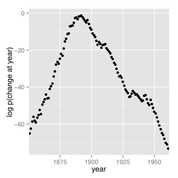
A plot of the values of $\log p(s \mid D)$ computed using Stan 2.4’s default MCMC implementation is shown in the posterior plot.

使用 Stan 2.4 默认的 MCMC 实现计算得到的 $\log p(s \mid D)$ 值的图示显示在后验图中。

Log probability of change point being in year, calculated analytically.

变点在年份上的对数概率，通过解析计算得到。

The frequency of change points generated by sampling the discrete change points.

通过对离散变点进行采样生成变点频率。

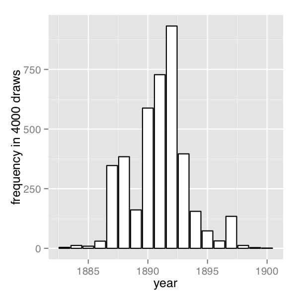
In order their range of estimates be visible, the first plot is on the log scale and the second plot on the linear scale; note the narrower range of years in the second plot resulting from sampling. The posterior mean of $s$ is roughly 1891.

为了使其估计范围可见，第一个图表使用对数尺度，第二个图表使用线性尺度；请注意，由于采样，第二个图表中年份的范围较窄。变点 s 的后验均值大约为1891年。

Discrete sampling

离散采样

The generated quantities block may be used to draw discrete parameter values using the built-in pseudo-random number generators. For example, with lp defined as above, the following program draws a random value for s at every iteration.

生成的量块可以使用内置的伪随机数生成器绘制离散参数值。例如，对于上述定义的 lp，以下程序在每次迭代中绘制 s 的随机值。

generated quantities {
  int<lower=1, upper=T> s;
  s = categorical_logit_rng(lp);
}

A posterior histogram of draws for $s$ is shown on the second change point posterior figure above.

在上面的第二个变点后验图中显示了对$s$的绘制的后验直方图。

Compared to working in terms of expectations, discrete sampling is highly inefficient, especially for tails of distributions, so this approach should only be used if draws from a distribution are explicitly required. Otherwise, expectations should be computed in the generated quantities block based on the posterior distribution for s given by softmax(lp).

与基于期望的方法相比，离散采样的计算效率较低，尤其是在处理分布尾部时。因此，只有在需要明确从分布中绘制样本时，才应使用此方法。否则，应根据由 softmax(lp) 给出的变点后验分布在生成的量块中计算期望值。

Posterior covariance

后验协方差

The discrete sample generated for $s$ can be used to calculate covariance with other parameters. Although the sampling approach is straightforward, it is more statistically efficient (in the sense of requiring far fewer iterations for the same degree of accuracy) to calculate these covariances in expectation using lp.

可以使用对 $s$ 进行的离散采样来计算与其他参数的协方差。虽然采样方法直观易懂，但使用 lp 计算这些协方差的期望值在统计效率上更优（即在相同精度要求下需要更少的迭代次数）。

Multiple change points

多变点

There is no obstacle in principle to allowing multiple change points. The only issue is that computation increases from linear to quadratic in marginalizing out two change points, cubic for three change points, and so on. There are three parameters, e, m, and l, and two loops for the change point and then one over time, with log densities being stored in a matrix.

原则上，允许多个变点是没有问题的。唯一的问题是，在将两个变点边缘化时，计算复杂度从线性增加到二次，三个变点则为立方形式，依此类推。有三个参数，e、m 和 l，以及两个循环，一个用于变点，另一个用于时间，其中对数密度存储在矩阵中。

matrix[T, T] lp;
lp = rep_matrix(log_unif, T);
for (s1 in 1:T) {
  for (s2 in 1:T) {
    for (t in 1:T) {
      lp[s1,s2] = lp[s1,s2]
        + poisson_lpmf(D[t] | t < s1 ? e : (t < s2 ? m : l));
    }
  }
}

The matrix can then be converted back to a vector using to_vector before being passed to log_sum_exp.

矩阵可以在传递给 log_sum_exp 之前使用 to_vector 转换回向量。

7.3 Mark-recapture models

标记-重捕模型

A widely applied field method in ecology is to capture (or sight) animals, mark them (e.g., by tagging), then release them. This process is then repeated one or more times, and is often done for populations on an ongoing basis. The resulting data may be used to estimate population size.

生态学中一种广泛应用的野外方法是捕捉（或观察）动物，给它们打上标记（例如标签），然后释放它们。然后，这个过程会重复一次或多次，并且通常会对种群进行持续的观测。得到的数据可以用于估计种群大小。

The first subsection describes a simple mark-recapture model that does not involve any latent discrete parameters. The following subsections describes the Cormack-Jolly-Seber model, which involves latent discrete parameters for animal death.

第一个小节描述了一个简单的标记-重捕模型，不涉及任何潜在的离散参数。接下来的小节描述了 Cormack-Jolly-Seber 模型，该模型涉及动物死亡的潜在离散参数。

Simple mark-recapture model

简单标记-重捕模型

In the simplest case, a one-stage mark-recapture study produces the following data

在最简单的情况下，一个一阶段的标记-重捕研究会产生以下数据：

$M$ : number of animals marked in first capture,
$C$ : number animals in second capture, and
$R$ : number of marked animals in second capture.
$M$：第一次捕捉时标记的动物数量，
$C$：第二次捕捉时的动物数量，
$R$：第二次捕捉时标记的动物数量。

The estimand of interest is

感兴趣的估计量是：

$N$ : number of animals in the population.
$N$：种群中的动物数量。

Despite the notation, the model will take $N$ to be a continuous parameter; just because the population must be finite doesn’t mean the parameter representing it must be. The parameter will be used to produce a real-valued estimate of the population size.

尽管符号表示为 $N$，但模型将将 $N$ 视为连续参数；尽管种群必须是有限的，但表示种群的参数并不一定是离散的。该参数将用于生成种群大小的一个实数估计。

The Lincoln-Petersen (Lincoln 1930; Petersen 1896) method for estimating population size is

Lincoln-Petersen 方法 (Lincoln 1930; Petersen 1896) 用于估计种群大小的公式为 \[ \hat{N} = \frac{M C}{R}. \]

This population estimate would arise from a probabilistic model in which the number of recaptured animals is distributed binomially,

这种种群估计是基于一个概率模型得出的，其中被重新捕获的动物数量服从二项分布，

\[ R \sim \textsf{binomial}(C, M / N) \] given the total number of animals captured in the second round ($C$) with a recapture probability of $M/N$, the fraction of the total population $N$ marked in the first round.

给定第二轮捕获的总动物数量（$C$）以及重新捕获概率 $M/N$，即第一轮标记的动物数量与总体 $N$ 的比例。

data {
  int<lower=0> M;
  int<lower=0> C;
  int<lower=0, upper=min(M, C)> R;
}
parameters {
  real<lower=(C - R + M)> N;
}
model {
  R ~ binomial(C, M / N);
}

A probabilistic formulation of the Lincoln-Petersen estimator for population size based on data from a one-step mark-recapture study. The lower bound on $N$ is necessary to efficiently eliminate impossible values.

Lincoln-Petersen 估计器的概率形式是基于一步标记-捕获研究的数据对种群大小进行估计。$N$ 的下界是必要的，以有效地排除不可能的值。

The probabilistic variant of the Lincoln-Petersen estimator can be directly coded in Stan as shown in the Lincon-Petersen model figure. The Lincoln-Petersen estimate is the maximum likelihood estimate (MLE) for this model.

Lincoln-Petersen 估计器的概率变体可以直接在 Stan 中编码，如 Lincoln-Petersen 模型图所示。Lincoln-Petersen 估计是该模型的最大似然估计（MLE）。

To ensure the MLE is the Lincoln-Petersen estimate, an improper uniform prior for $N$ is used; this could (and should) be replaced with a more informative prior if possible, based on knowledge of the population under study.

为确保 MLE 是 Lincoln-Petersen 估计，对 $N$ 使用了非正规的均匀先验分布；如果可能的话，应该根据对研究种群的了解，用更具信息的先验进行替代。

The one tricky part of the model is the lower bound $C - R + M$ placed on the population size $N$. Values below this bound are impossible because it is otherwise not possible to draw $R$ samples out of the $C$ animals recaptured. Implementing this lower bound is necessary to ensure sampling and optimization can be carried out in an unconstrained manner with unbounded support for parameters on the transformed (unconstrained) space. The lower bound in the declaration for $C$ implies a variable transform $f : (C-R+M,\infty) \rightarrow (-\infty,+\infty)$ defined by $f(N) = \log(N - (C - R + M))$; the reference manual contains full details of all constrained parameter transforms.

模型中的一个棘手部分是对种群大小 $N$ 设置的下界 $C - R + M$。低于此下界的值是不可能的，因为否则无法从重新捕获的 $C$ 只动物中抽取 $R$ 个样本。实现此下界是为了确保在变换后的（非约束）空间上的参数支持无界，使得采样和优化能够以非约束的方式进行。在 $C$ 的声明中的下界意味着一个变量变换 $f : (C-R+M,\infty) \rightarrow (-\infty,+\infty)$，其中 $f(N) = \log(N - (C - R + M))$；参考手册中包含了所有约束参数变换的详细信息。

Cormack-Jolly-Seber with discrete parameter

具有离散参数的 Cormack-Jolly-Seber 模型

The Cormack-Jolly-Seber (CJS) model (Cormack 1964; Jolly 1965; Seber 1965) is an open-population model in which the population may change over time due to death; the presentation here draws heavily on Schofield (2007).

Cormack-Jolly-Seber (CJS) 模型 (Cormack 1964; Jolly 1965; Seber 1965) 是一个开放种群模型，种群可能随时间发生变化，原因是死亡；这里的介绍主要参考了 Schofield (2007)。

The basic data are

基本数据包括：

$I$: number of individuals,
$T$: number of capture periods, and
$y_{i,t}$: Boolean indicating if individual $i$ was captured at time $t$.
$I$：个体数量，
$T$：捕获期数，
$y_{i,t}$：布尔值，指示个体$i$是否在时间$t$被捕获。

Each individual is assumed to have been captured at least once because an individual only contributes information conditionally after they have been captured the first time.

假设每个个体至少被捕获一次，因为只有在个体第一次被捕获后，它们才能提供有条件的信息。

There are two Bernoulli parameters in the model,

模型中有两个伯努利参数：

$\phi_t$ : probability that animal alive at time $t$ survives until $t + 1$ and
$p_t$ : probability that animal alive at time $t$ is captured at time $t$.
$\phi_t$：在时间 $t$ 时存活的动物在 $t+1$ 时存活的概率，
$p_t$：在时间 $t$ 时存活的动物在时间 $t$ 时被捕获的概率。

These parameters will both be given uniform priors, but information should be used to tighten these priors in practice.

这些参数都将具有均匀先验分布，但在实践中应使用信息来加优化这些先验分布。

The CJS model also employs a latent discrete parameter $z_{i,t}$ indicating for each individual $i$ whether it is alive at time $t$, distributed as

CJS 模型还使用了一个隐含的离散参数 $z_{i,t}$，用于指示每个个体 $i$ 在时间 $t$ 是否存活，其分布为 \[ z_{i,t} \sim \mathsf{Bernoulli}(z_{i,t-1} \; ? \; 0 \: : \: \phi_{t-1}). \]

The conditional prevents the model positing zombies; once an animal is dead, it stays dead. The data distribution is then simple to express conditional on $z$ as

这个条件约束防止了模型中出现“僵尸”动物的情况；一旦动物死亡，它将保持死亡状态。在给定 $z$ 的条件下，数据分布可以简单地表示为

\[ y_{i,t} \sim \mathsf{Bernoulli}(z_{i,t} \; ? \; 0 \: : \: p_t). \]

The conditional enforces the constraint that dead animals cannot be captured.

这个条件约束确保了已死亡的动物无法被捕获。

Collective Cormack-Jolly-Seber model

群体 Cormack-Jolly-Seber 模型

This subsection presents an implementation of the model in terms of counts for different history profiles for individuals over three capture times. It assumes exchangeability of the animals in that each is assigned the same capture and survival probabilities.

本小节介绍了一种根据个体在三个捕获时间段内的历史配置进行计数的模型实现。该模型假设动物之间是可交换的，每个动物具有相同的捕获和存活概率。

In order to ease the marginalization of the latent discrete parameter $z_{i,t}$, the Stan models rely on a derived quantity $\chi_t$ for the probability that an individual is never captured again if it is alive at time $t$ (if it is dead, the recapture probability is zero). this quantity is defined recursively by

为了简化对潜在离散参数 $z_{i,t}$ 的边际化处理，Stan 模型依赖于一个派生量 $\chi_t$，用于表示在时间 $t$ 仍然存活的个体再次被捕获的概率（如果个体已经死亡，则再次捕获概率为零）。该数量通过递归方式定义如下： \[ \chi_t = \begin{cases} 1 & \quad\text{if } t = T \\ (1 - \phi_t) + \phi_t (1 - p_{t+1}) \chi_{t+1} & \quad\text{if } t < T \end{cases} \]

The base case arises because if an animal was captured in the last time period, the probability it is never captured again is 1 because there are no more capture periods. The recursive case defining $\chi_{t}$ in terms of $\chi_{t+1}$ involves two possibilities: (1) not surviving to the next time period, with probability $(1 - \phi_t)$, or (2) surviving to the next time period with probability $\phi_t$, not being captured in the next time period with probability $(1 - p_{t+1})$, and not being captured again after being alive in period $t+1$ with probability $\chi_{t+1}$.

基本情况是，如果动物在最后一个时间段被捕获，那么它再次被捕获的概率为1，因为没有更多的捕获时间段。根据 $\chi_{t+1}$ 定义 $\chi_{t}$ 的递归情况包括两种可能性：(1) 不在下一个时间段存活的概率为 $(1-\phi_t)$；(2) 在下一个时间段存活的概率为 $\phi_t$，在下一个时间段未被捕获的概率为 $(1-p_{t+1})$，并且在 $t+1$ 期后继续存活的概率为 $\chi_{t+1}$。

With three capture times, there are eight captured/not-captured profiles an individual may have. These may be naturally coded as binary numbers as follows.

对于三个捕获时间段，个体可能具有八种被捕获/未被捕获的配置。这些可以自然地编码为二进制数，如下所示。

\[ \begin{array}{crclc} \hline & \qquad\qquad & captures & \qquad\qquad & \\ \mathrm{profile} & 1 & 2 & 3 & \mathrm{probability} \\ \hline 0 & - & - & - & n/a \\ 1 & - & - & + & n/a \\ 2 & - & + & - & \chi_2 \\ 3 & - & + & + & \phi_2 \, p_3 \\ 4 & + & - & - & \chi_1 \\ 5 & + & - & + & \phi_1 \, (1 - p_2) \, \phi_2 \, p_3 \\ 6 & + & + & - & \phi_1 \, p_2 \, \chi_2 \\ 7 & + & + & + & \phi_1 \, p_2 \, \phi_2 \, p_3 \\ \hline \end{array} \]

History 0, for animals that are never captured, is unobservable because only animals that are captured are observed. History 1, for animals that are only captured in the last round, provides no information for the CJS model, because capture/non-capture status is only informative when conditioned on earlier captures. For the remaining cases, the contribution to the likelihood is provided in the final column.

对于从未被捕获的动物，其历史记录为0，因为只有被捕获的动物才能被观察到。对于仅在最后一轮被捕获的动物，它们对 CJS 模型没有提供任何信息，因为捕获/未捕获的状态只有在先前的捕获条件下才具有信息价值。对于其余情况，对似然函数的贡献在最后一列中给出。

By defining these probabilities in terms of $\chi$ directly, there is no need for a latent binary parameter indicating whether an animal is alive at time $t$ or not. The definition of $\chi$ is typically used to define the likelihood (i.e., marginalize out the latent discrete parameter) for the CJS model (Schofield 2007).

通过直接基于 $\chi$ 来定义这些概率，就不需要使用一个潜在的二进制参数来指示动物在时间 $t$ 是否存活。$\chi$ 的定义通常用于定义 CJS 模型的似然函数（即边际化潜在离散参数）。

The Stan model defines $\chi$ as a transformed parameter based on parameters $\phi$ and $p$. In the model block, the log probability is incremented for each history based on its count. This second step is similar to collecting Bernoulli observations into a binomial or categorical observations into a multinomial, only it is coded directly in the Stan program using target += rather than being part of a built-in probability function.

Stan 模型将 $\chi$ 定义为基于参数 $\phi$ 和 $p$ 的转换参数。在模型块中，根据每个历史的计数递增对数概率。这第二步类似于将伯努利观测值汇总为二项式或将分类观测值汇总为多项式，只是在 Stan 程序中直接使用 target += 进行编码，而不是作为内置概率函数的一部分。

The following is the Stan program for the Cormack-Jolly-Seber mark-recapture model that considers counts of individuals with observation histories of being observed or not in three capture periods

以下是考虑个体在三个捕获时间段内被观察或未被观察的历史计数的 Cormack-Jolly-Seber 标记-再捕获模型的 Stan 程序：

data {
  array[7] int<lower=0> history;
}
parameters {
  array[2] real<lower=0, upper=1> phi;
  array[3] real<lower=0, upper=1> p;
}
transformed parameters {
  array[2] real<lower=0, upper=1> chi;
  chi[2] = (1 - phi[2]) + phi[2] * (1 - p[3]);
  chi[1] = (1 - phi[1]) + phi[1] * (1 - p[2]) * chi[2];
}
model {
  target += history[2] * log(chi[2]);
  target += history[3] * (log(phi[2]) + log(p[3]));
  target += history[4] * (log(chi[1]));
  target += history[5] * (log(phi[1]) + log1m(p[2])
                            + log(phi[2]) + log(p[3]));
  target += history[6] * (log(phi[1]) + log(p[2])
                            + log(chi[2]));
  target += history[7] * (log(phi[1]) + log(p[2])
                            + log(phi[2]) + log(p[3]));
}
generated quantities {
  real<lower=0, upper=1> beta3;
  beta3 = phi[2] * p[3];
}

Identifiability

可辨识性

The parameters $\phi_2$ and $p_3$, the probability of death at time 2 and probability of capture at time 3 are not identifiable, because both may be used to account for lack of capture at time 3. Their product, $\beta_3 = \phi_2 \, p_3$, is identified. The Stan model defines beta3 as a generated quantity. Unidentified parameters pose a problem for Stan’s samplers’ adaptation. Although the problem posed for adaptation is mild here because the parameters are bounded and thus have proper uniform priors, it would be better to formulate an identified parameterization. One way to do this would be to formulate a hierarchical model for the $p$ and $\phi$ parameters.

参数 $\phi_2$ 和$p_3$，即时间2的死亡概率和时间3的捕获概率，是不可辨识的，因为两者都可以用来解释在时间3没有捕获到的情况。它们的乘积 $\beta_3 = \phi_2 \, p_3$ 是可辨识的。Stan 模型将 beta3 定义为生成的数量。不可辨识的参数对于 Stan 抽样器的自适应性会出问题。虽然在这里对自适应性的问题较小，因为参数是有界的，因此具有适当的均匀先验分布，但更好的做法是制定一个可辨识的参数化模型。一种方法是为 $p$ 和 $\phi$ 参数制定一个分层模型。

Individual Cormack-Jolly-Seber model

个体级 Cormack-Jolly-Seber 模型

This section presents a version of the Cormack-Jolly-Seber (CJS) model cast at the individual level rather than collectively as in the previous subsection. It also extends the model to allow an arbitrary number of time periods. The data will consist of the number $T$ of capture events, the number $I$ of individuals, and a boolean flag $y_{i,t}$ indicating if individual $i$ was observed at time $t$. In Stan,

本节介绍的是 Cormack-Jolly-Seber（CJS）模型的个体级别版本，而非前一小节中的群体级别模型。它还扩展了模型，允许任意数量的时间段。数据包括捕获事件数量 $T$，个体数量 $I$，以及一个布尔标志 $y_{i,t}$，指示个体 $i$ 是否在时间 $t$ 被观察到。在 Stan 中，

data {
  int<lower=2> T;
  int<lower=0> I;
  array[I, T] int<lower=0, upper=1> y;
}

The advantages to the individual-level model is that it becomes possible to add individual “random effects” that affect survival or capture probability, as well as to avoid the combinatorics involved in unfolding $2^T$ observation histories for $T$ capture times.

个体级别模型的优势在于能够引入影响存活或捕获概率的个体“随机效应”，同时避免了在展开 $2^T$ 个观测历史（对应于 $T$ 个捕获时间）时涉及的组合问题。

Utility functions

效用函数

The individual CJS model is written involves several function definitions. The first two are used in the transformed data block to compute the first and last time period in which an animal was captured.⁷

个体级 CJS 模型包含几个函数定义。前两个函数用于在转换数据块中计算动物被捕获的第一个和最后一个时间点。⁸

functions {
  int first_capture(array[] int y_i) {
    for (k in 1:size(y_i)) {
      if (y_i[k]) {
        return k;
      }
    }
    return 0;
  }
  int last_capture(array[] int y_i) {
    for (k_rev in 0:(size(y_i) - 1)) {
      int k;
      k = size(y_i) - k_rev;
      if (y_i[k]) {
        return k;
      }
    }
    return 0;
  }
  // ...
}

These two functions are used to define the first and last capture time for each individual in the transformed data block.⁹

这两个函数用于在转换的数据块中定义每个个体的第一个和最后一个捕获时间。¹⁰

transformed data {
  array[I] int<lower=0, upper=T> first;
  array[I] int<lower=0, upper=T> last;
  vector<lower=0, upper=I>[T] n_captured;
  for (i in 1:I) {
    first[i] = first_capture(y[i]);
  }
  for (i in 1:I) {
    last[i] = last_capture(y[i]);
  }
  n_captured = rep_vector(0, T);
  for (t in 1:T) {
    for (i in 1:I) {
      if (y[i, t]) {
        n_captured[t] = n_captured[t] + 1;
      }
    }
  }
}

The transformed data block also defines n_captured[t], which is the total number of captures at time t. The variable n_captured is defined as a vector instead of an integer array so that it can be used in an elementwise vector operation in the generated quantities block to model the population estimates at each time point.

转换数据块还定义了 n_captured[t]，表示在时间点 t 的总捕获次数。变量 n_captured 被定义为一个向量而不是整数数组，以便在生成的数量块中可以将其用于元素级的向量操作，从而对每个时间点的种群估计进行建模。

The parameters and transformed parameters are as before, but now there is a function definition for computing the entire vector chi, the probability that if an individual is alive at t that it will never be captured again.

参数和转换参数与之前一致，但现在增加了一个函数定义，用于计算整个向量 chi，表示如果个体在时间点 t 仍然存活，则它将永远不会再次被捕获的概率。

parameters {
  vector<lower=0, upper=1>[T - 1] phi;
  vector<lower=0, upper=1>[T] p;
}
transformed parameters {
  vector<lower=0, upper=1>[T] chi;
  chi = prob_uncaptured(T, p, phi);
}

The definition of prob_uncaptured, from the functions block, is

prob_uncaptured 的定义来自函数块，如下所示：

functions {
  // ...
  vector prob_uncaptured(int T, vector p, vector phi) {
    vector[T] chi;
    chi[T] = 1.0;
    for (t in 1:(T - 1)) {
      int t_curr;
      int t_next;
      t_curr = T - t;
      t_next = t_curr + 1;
      chi[t_curr] = (1 - phi[t_curr])
                     + phi[t_curr]
                       * (1 - p[t_next])
                       * chi[t_next];
    }
    return chi;
  }
}

The function definition directly follows the mathematical definition of $\chi_t$, unrolling the recursion into an iteration and defining the elements of chi from T down to 1.

函数定义直接按照 $\chi_t$ 的数学定义进行，将递归展开为迭代，并从 T 到1定义了 chi 的元素。

The model

模型

Given the precomputed quantities, the model block directly encodes the CJS model’s log likelihood function. All parameters are left with their default uniform priors and the model simply encodes the log probability of the observations q given the parameters p and phi as well as the transformed parameter chi defined in terms of p and phi.

基于预先计算的量，模型块直接编码了 CJS 模型的对数似然函数。所有参数均保留其默认的均匀先验分布，模型简单地编码了在给定参数 p 和 phi 以及以 p 和 phi 定义的变换参数 chi 的情况下，观测值 q 的对数概率。

model {
  for (i in 1:I) {
    if (first[i] > 0) {
      for (t in (first[i]+1):last[i]) {
        1 ~ bernoulli(phi[t - 1]);
        y[i, t] ~ bernoulli(p[t]);
      }
      1 ~ bernoulli(chi[last[i]]);
    }
  }
}

The outer loop is over individuals, conditional skipping individuals i which are never captured. The never-captured check depends on the convention of the first-capture and last-capture functions returning 0 for first if an individual is never captured.

外部循环遍历所有个体，条件是跳过从未被捕获的个体 i。判断个体是否从未被捕获依赖于第一次捕获和最后一次捕获函数对于未被捕获的个体返回0的约定。

The inner loop for individual i first increments the log probability based on the survival of the individual with probability phi[t - 1]. The outcome of 1 is fixed because the individual must survive between the first and last capture (i.e., no zombies). The loop starts after the first capture, because all information in the CJS model is conditional on the first capture.

个体 i 的内部循环首先根据个体的存活概率 phi[t - 1] 增加对数概率。结果为1是固定的，因为个体必须在第一次和最后一次捕获之间存活（即不存在僵尸）。循环从第一次捕获后开始，因为 CJS 模型中的所有信息都是以第一次捕获为条件的。

In the inner loop, the observed capture status y[i, t] for individual i at time t has a Bernoulli distribution based on the capture probability p[t] at time t.

在内部循环中，个体 i 在时间点 t 的观测捕获状态 y[i, t] 服从基于时间点 t 的捕获概率 p[t] 的伯努利分布。

After the inner loop, the probability of an animal never being seen again after being observed at time last[i] is included, because last[i] was defined to be the last time period in which animal i was observed.

在内部循环之后，还计算了个体 i 在时间点 last[i] 被观察后再也没有被捕获的概率，因为 last[i] 被定义为个体 i 最后一次被观察到的时间点。

Identified parameters

识别参数

As with the collective model described in the previous subsection, this model does not identify phi[T - 1] and p[T], but does identify their product, beta. Thus beta is defined as a generated quantity to monitor convergence and report.

与前面小节描述的群体模型类似，该模型无法单独确定 phi[T - 1] 和 p[T]，但可以确定它们的乘积 beta。因此，beta 被定义为生成的量，用于监测收敛性和报告。

generated quantities {
  real beta;
  // ...

  beta = phi[T - 1] * p[T];
  // ...
}

The parameter p[1] is also not modeled and will just be uniform between 0 and 1. A more finely articulated model might have a hierarchical or time-series component, in which case p[1] would be an unknown initial condition and both phi[T - 1] and p[T] could be identified.

参数 p[1] 也没有建模，并且仅在0到1之间均匀分布。一个更细致的模型可能会包含层次或时间序列的组成部分，此时 p[1] 将是一个未知的初始条件，并且phi[T - 1] 和 p[T] 都可以确定。

Population size estimates

人口规模估计

The generated quantities also calculates an estimate of the population mean at each time t in the same way as in the simple mark-recapture model as the number of individuals captured at time t divided by the probability of capture at time t. This is done with the elementwise division operation for vectors (./) in the generated quantities block.

在生成量中，还计算了每个时间点 t 的种群均值估计，方法与简单标记-重捕模型相同，即将时间点 t 捕获的个体数除以时间点 t 的捕获概率。这是通过向量的元素级除法操作（./）在生成的量块中完成的。

generated quantities {
  // ...
  vector<lower=0>[T] pop;
  // ...
  pop = n_captured ./ p;
  pop[1] = -1;
}

Generalizing to individual effects

个体效应的泛化

All individuals are modeled as having the same capture probability, but this model could be easily generalized to use a logistic regression here based on individual-level inputs to be used as predictors.

所有个体被建模为具有相同的捕获概率，但该模型可以轻松扩展为基于个体级别输入的 Logistic 回归模型，作为预测变量。

7.4 Data coding and diagnostic accuracy models

数据编码和诊断准确性模型

Although seemingly disparate tasks, the rating/coding/annotation of items with categories and diagnostic testing for disease or other conditions, share several characteristics which allow their statistical properties to be modeled similarly.

尽管看似不相关的任务，但对物品进行分类和编码以及对疾病或其他状况进行诊断测试具有相似的特征，使得它们的统计属性可以以类似的方式建模。

Diagnostic accuracy

诊断准确性

Suppose you have diagnostic tests for a condition of varying sensitivity and specificity. Sensitivity is the probability a test returns positive when the patient has the condition and specificity is the probability that a test returns negative when the patient does not have the condition. For example, mammograms and puncture biopsy tests both test for the presence of breast cancer. Mammograms have high sensitivity and low specificity, meaning lots of false positives, whereas puncture biopsies are the opposite, with low sensitivity and high specificity, meaning lots of false negatives.

假设你已经针对某种病症具有不同敏感性和特异性的诊断测试。敏感性是指当患者患有该病症时，测试结果呈阳性的概率；特异性是指当患者没有该病症时，测试结果呈阴性的概率。例如，乳腺X线摄影和穿刺活检都用于检测乳腺癌的存在。乳腺X线摄影具有较高的敏感性和较低的特异性，意味着存在很多假阳性结果，而穿刺活检则相反，具有较低的敏感性和较高的特异性，意味着存在很多假阴性结果。

There are several estimands of interest in such studies. An epidemiological study may be interested in the prevalence of a kind of infection, such as malaria, in a population. A test development study might be interested in the diagnostic accuracy of a new test. A health care worker performing tests might be interested in the disease status of a particular patient.

这类研究中存在几个感兴趣的估计量。在流行病学研究中，可能对人群中某种感染（如疟疾）的患病率感兴趣。测试开发研究可能对新测试的诊断准确性感兴趣。执行测试的医护人员可能对特定患者的疾病状态感兴趣。

Data coding

数据编码

Humans are often given the task of coding (equivalently rating or annotating) data. For example, journal or grant reviewers rate submissions, a political study may code campaign commercials as to whether they are attack ads or not, a natural language processing study might annotate Tweets as to whether they are positive or negative in overall sentiment, or a dentist looking at an X-ray classifies a patient as having a cavity or not. In all of these cases, the data coders play the role of the diagnostic tests and all of the same estimands are in play — data coder accuracy and bias, true categories of items being coded, or the prevalence of various categories of items in the data.

通常需要人类来对数据进行编码（也可以称为评级或注释）。例如，期刊或拨款评审人员对提交的稿件进行评级，政治研究可能对竞选广告进行编码，判断其是否是攻击性广告，自然语言处理研究可能对推文进行注释，判断其整体情感是积极还是消极，牙医在查看X光片时对患者进行龋齿与否的分类。在所有这些情况下，数据编码者扮演着诊断测试的角色，并且所有相同的估计量都适用——数据编码者的准确性和偏差，被编码的项目的真实类别，以及数据中各类别项目的患病率。

Noisy categorical measurement model

嘈杂的分类测量模型

In this section, only categorical ratings are considered, and the challenge in the modeling for Stan is to marginalize out the discrete parameters.

在本节中，只考虑分类评级，并且 Stan 建模的挑战是要边缘化离散参数。

Dawid and Skene (1979) introduce a noisy-measurement model for coding and apply it in the epidemiological setting of coding what doctors say about patient histories; the same model can be used for diagnostic procedures.

Dawid and Skene (1979) 引入了一种嘈杂测量模型用于编码，并将其应用于编码医生对患者病史所说内容的流行病学设置中；相同的模型也可以用于诊断程序。

Data

数据

The data for the model consists of $J$ raters (diagnostic tests), $I$ items (patients), and $K$ categories (condition statuses) to annotate, with $y_{i, j} \in \{1, \dotsc, K\}$ being the rating provided by rater $j$ for item $i$. In a diagnostic test setting for a particular condition, the raters are diagnostic procedures and often $K=2$, with values signaling the presence or absence of the condition.¹¹

该模型的数据包括 $J$ 个评级者（诊断测试）、$I$ 个项目（患者）和 $K$ 个要进行注释的类别（疾病状态），其中 $y_{i,j} \in \{1, \dotsc, K\}$ 表示评级者 $j$ 对项目 $i$ 的评级。在特定疾病的诊断测试环境中，评级者通常是诊断程序，而 $K=2$，表示疾病的存在与否。¹²

It is relatively straightforward to extend Dawid and Skene’s model to deal with the situation where not every rater rates each item exactly once.

将 Dawid 和 Skene 的模型扩展到不是每个评级者都对每个项目进行精确评级的情况相对简单。

Model parameters

模型参数

The model is based on three parameters, the first of which is discrete:

该模型基于三个参数，其中第一个是离散的：

$z_i$ : a value in $\{1, \dotsc, K\}$ indicating the true category of item $i$,
$\pi$ : a $K$-simplex for the prevalence of the $K$ categories in the population, and
$\theta_{j,k}$ : a $K$-simplex for the response of annotator $j$ to an item of true category $k$.
$z_i$：取值为 $\{1, \dotsc, K\}$ 的变量，表示项目 $i$ 的真实类别，
$\pi$：$K$-simplex，表示人群中 $K$ 个类别的流行度分布，
$\theta_{j,k}$：$K$-simplex，表示评级者 $j$ 对真实类别为 $k$ 的项目的反应。

Noisy measurement model

噪声测量模型

The true category of an item is assumed to be generated by a simple categorical distribution based on item prevalence,

假设项目的真实类别是根据项目流行度的简单分类分布生成的， \[ z_i \sim \textsf{categorical}(\pi). \]

The rating $y_{i, j}$ provided for item $i$ by rater $j$ is modeled as a categorical response of rater $i$ to an item of category $z_i$,¹³

评级者 $j$ 对项目 $i$ 提供的评级 $y_{i, j}$ 被建模为评级者 $j$ 对类别为 $z_i$ 的项目的分类响应。¹⁴ \[ y_{i, j} \sim \textsf{categorical}(\theta_{j,\pi_{z[i]}}). \]

Priors and hierarchical modeling

先验和分层建模

Dawid and Skene provided maximum likelihood estimates for $\theta$ and $\pi$, which allows them to generate probability estimates for each $z_i$.

Dawid 和 Skene 提供了 $\theta$ 和 $\pi$ 的最大似然估计，使他们能够为每个 $z_i$ 生成概率估计。

To mimic Dawid and Skene’s maximum likelihood model, the parameters $\theta_{j,k}$ and $\pi$ can be given uniform priors over $K$-simplexes. It is straightforward to generalize to Dirichlet priors,

为了模仿 Dawid 和 Skene 的最大似然模型，可以给参数 $\theta_{j,k}$ 和 $\pi$ 一个 $K$-simplex 的均匀先验。可以将其一般化为狄利克雷先验： \[ \pi \sim \textsf{Dirichlet}(\alpha) \] and

和 \[ \theta_{j,k} \sim \textsf{Dirichlet}(\beta_k) \] with fixed hyperparameters $\alpha$ (a vector) and $\beta$ (a matrix or array of vectors). The prior for $\theta_{j,k}$ must be allowed to vary in $k$, so that, for instance, $\beta_{k,k}$ is large enough to allow the prior to favor better-than-chance annotators over random or adversarial ones.

其中 $\alpha$（一个向量）和 $\beta$（一个矩阵或向量数组）是固定的超参数。$\theta_{j,k}$ 的先验必须在 $k$ 上是可变的，以便例如 $\beta_{k,k}$ 足够大，使得先验能够偏好优于随机或对抗性的评级者。

Because there are $J$ coders, it would be natural to extend the model to include a hierarchical prior for $\beta$ and to partially pool the estimates of coder accuracy and bias.

由于存在 $J$ 个编码者，自然可以扩展模型，为 $\beta$ 包含一个分层先验，并部分共享编码者准确性和偏差的估计。

Marginalizing out the true category

边缘化真实类别

Because the true category parameter $z$ is discrete, it must be marginalized out of the joint posterior in order to carry out sampling or maximum likelihood estimation in Stan. The joint posterior factors as

由于真实类别参数 $z$ 是离散的，为了在 Stan 中进行抽样或最大似然估计，必须将其从联合后验中边缘化出来。联合后验可分解为： \[ p(y, \theta, \pi) = p(y \mid \theta,\pi) \, p(\pi) \, p(\theta), \] where $p(y \mid \theta,\pi)$ is derived by marginalizing $z$ out of

其中 $p(y \mid \theta,\pi)$ 是通过对 $z$ 进行边际化得到的。 \[ p(z, y \mid \theta, \pi) = \prod_{i=1}^I \left( \textsf{categorical}(z_i \mid \pi) \prod_{j=1}^J \textsf{categorical}(y_{i, j} \mid \theta_{j, z[i]}) \right). \]

This can be done item by item, with

可以逐个项目进行计算，得到边缘化的概率：

\[ p(y \mid \theta, \pi) = \prod_{i=1}^I \sum_{k=1}^K \left( \textsf{categorical}(k \mid \pi) \prod_{j=1}^J \textsf{categorical}(y_{i, j} \mid \theta_{j, k}) \right). \]

In the missing data model, only the observed labels would be used in the inner product.

在缺失数据模型中，只有观测到的标签会在内积中使用。

Dawid and Skene (1979) derive exactly the same equation in their Equation (2.7), required for the E-step in their expectation maximization (EM) algorithm. Stan requires the marginalized probability function on the log scale,

Dawid and Skene (1979) 在他们的期望最大化（EM）算法的 E 步中，推导出了完全相同的方程（2.7）。在 Stan 中，需要对边际化的概率函数进行对数变换。

\[\begin{align*} \log p(y \mid \theta, \pi) &= \sum_{i=1}^I \log \left( \sum_{k=1}^K \exp \left(\log \textsf{categorical}(k \mid \pi) \vphantom{\sum_{j=1}^J}\right.\right. \left.\left. + \ \sum_{j=1}^J \log \textsf{categorical}(y_{i, j} \mid \theta_{j, k}) \right) \right), \end{align*}\] which can be directly coded using Stan’s built-in log_sum_exp function.

这可以直接使用Stan内置的log_sum_exp函数进行编码。

Stan implementation

Stan 实现

The Stan program for the Dawid and Skene model is provided below (Dawid and Skene 1979).

以下是 Dawid 和 Skene 模型的 Stan 程序实现(Dawid and Skene 1979)。

data {
  int<lower=2> K;
  int<lower=1> I;
  int<lower=1> J;

  array[I, J] int<lower=1, upper=K> y;

  vector<lower=0>[K] alpha;
  vector<lower=0>[K] beta[K];
}
parameters {
  simplex[K] pi;
  array[J, K] simplex[K] theta;
}
transformed parameters {
  array[I] vector[K] log_q_z;
  for (i in 1:I) {
    log_q_z[i] = log(pi);
    for (j in 1:J) {
      for (k in 1:K) {
        log_q_z[i, k] = log_q_z[i, k]
                         + log(theta[j, k, y[i, j]]);
      }
    }
  }
}
model {
  pi ~ dirichlet(alpha);
  for (j in 1:J) {
    for (k in 1:K) {
      theta[j, k] ~ dirichlet(beta[k]);
    }
  }

  for (i in 1:I) {
    target += log_sum_exp(log_q_z[i]);
  }
}

The model marginalizes out the discrete parameter $z$, storing the unnormalized conditional probability $\log q(z_i=k|\theta,\pi)$ in log_q_z[i, k].

模型通过边缘化离散参数 $z$，将未标准化的条件概率 $\log q(z_i=k|\theta,\pi)$ 存储在 log_q_z[i, k] 中。

The Stan model converges quickly and mixes well using NUTS starting at diffuse initial points, unlike the equivalent model implemented with Gibbs sampling over the discrete parameter. Reasonable weakly informative priors are $\alpha_k = 3$ and $\beta_{k,k} = 2.5 K$ and $\beta_{k,k'} = 1$ if $k \neq k'$. Taking $\alpha$ and $\beta_k$ to be unit vectors and applying optimization will produce the same answer as the expectation maximization (EM) algorithm of Dawid and Skene (1979).

使用 NUTS 从模糊的初始点开始，Stan 模型收敛迅速且混合效果良好，而使用 Gibbs 采样的等价模型无法达到相同的效果。合理的弱信息先验为 $\alpha_k = 3$ 和 $\beta_{k,k} = 2.5 K$，以及如果 $k \neq k'$，则 $\beta_{k,k'} = 1$。将 $\alpha$ 和 $\beta_k$ 视为单位向量，并应用优化，将得到与 Dawid and Skene (1979) 的期望最大化（EM）算法相同的结果。

Inference for the true category

对真实类别的推断

The quantity log_q_z[i] is defined as a transformed parameter. It encodes the (unnormalized) log of $p(z_i \mid \theta, \pi)$. Each iteration provides a value conditioned on that iteration’s values for $\theta$ and $\pi$. Applying the softmax function to log_q_z[i] provides a simplex corresponding to the probability mass function of $z_i$ in the posterior. These may be averaged across the iterations to provide the posterior probability distribution over each $z_i$.

log_q_z[i] 被定义为一个转换参数。它编码了基于 $\theta$ 和 $\pi$ 的 $p(z_i \mid \theta, \pi)$ 的（未标准化的）对数。每次迭代都会提供一个值，该值基于该迭代对 $\theta$ 和 $\pi$ 的值进行条件化。对 log_q_z[i] 应用 softmax 函数会提供与后验中 $z_i$ 的概率质量函数相对应的单纯形。可以对这些值进行迭代平均，以获得关于每个 $z_i$ 的后验概率分布。

7.5 The mathematics of recovering marginalized parameters

从边缘化模型中恢复边缘化参数的数学原理

Introduction

引言

This section describes in more detail the mathematics of statistical inference using the output of marginalized Stan models, such as those presented in the last three sections. It provides a mathematical explanation of why and how certain manipulations of Stan’s output produce valid summaries of the posterior distribution when discrete parameters have been marginalized out of a statistical model. Ultimately, however, fully understanding the mathematics in this section is not necessary to fit models with discrete parameters using Stan.

本节详细介绍了使用边缘化 Stan 模型的输出进行统计推断的数学原理，例如前三节中介绍的模型。它提供了关于为什么以及如何对 Stan 的输出进行某些操作以产生后验分布的有效摘要的数学解释，当统计模型中的离散参数被边缘化时。然而，完全理解本节中的数学内容不是使用 Stan 拟合具有离散参数的模型所必需的。

Throughout, the model under consideration consists of both continuous parameters, $\Theta$, and discrete parameters, $Z$. It is also assumed that $Z$ can only take finitely many values, as is the case for all the models described in this chapter of the User’s Guide. To simplify notation, any conditioning on data is suppressed in this section, except where specified. As with all Bayesian analyses, however, all inferences using models with marginalized parameters are made conditional on the observed data.

在整个过程中，所考虑的模型包括连续参数 $\Theta$ 和离散参数 $Z$。同时假设 $Z$ 只能取有限个值，这是用户指南本章中描述的所有模型的情况。为了简化符号表示，除非另有说明，在本节中省略了对数据的条件约束。然而，与所有贝叶斯分析一样，使用具有边缘化参数的模型进行的所有推断都是基于观测数据的条件推断。

Estimating expectations

估计期望值

When performing Bayesian inference, interest often centers on estimating some (constant) low-dimensional summary statistics of the posterior distribution. Mathematically, we are interested in estimating $\mu$, say, where $\mu = \mathbb{E}[g(\Theta, Z)]$ and $g(\cdot)$ is an arbitrary function. An example of such a quantity is $\mathbb{E}[\Theta]$, the posterior mean of the continuous parameters, where we would take $g(\theta, z) = \theta$. To estimate $\mu$ the most common approach is to sample a series of values, at least approximately, from the posterior distribution of the parameters of interest. The numerical values of these draws can then be used to calculate the quantities of interest. Often, this process of calculation is trivial, but more care is required when working with marginalized posteriors as we describe in this section.

在进行贝叶斯推断时，通常关注的是估计后验分布的某些（常数维度的）概括统计量。数学上，我们对估计 $\mu$ 感兴趣，其中 $\mu = \mathbb{E}[g(\Theta, Z)]$，$g(\cdot)$ 是任意函数。一个例子是 $\mathbb{E}[\Theta]$，即连续参数的后验均值，其中我们可以取 $g(\theta, z) = \theta$。为了估计 $\mu$，最常见的方法是从感兴趣的参数的后验分布中采样一系列值（至少近似地）。然后可以使用这些抽样的数值来计算感兴趣的量。通常，这个计算过程很简单，但在处理边缘化后验时需要更加小心，正如我们在本节中所描述的。

If both $\Theta$ and $Z$ were continuous, Stan could be used to sample $M$ draws from the joint posterior $p_{\Theta, Z}(\theta, z)$ and then estimate $\mu$ with

如果 $\Theta$ 和 $Z$ 都是连续的，可以使用 Stan 从联合后验分布 $p_{\Theta, Z}(\theta, z)$ 中采样 $M$ 个值，然后使用以下估计量来估计 $\mu$：

\[ \] = _{i = 1}^M {g(^{(i)}, z^{(i)})}. $$ Given $Z$ is discrete, however, Stan cannot be used to sample from the joint posterior (or even to do optimization). Instead, as outlined in the previous sections describing specific models, the user can first marginalize out $Z$ from the joint posterior to give the marginalized posterior $p_\Theta(\theta)$. This marginalized posterior can then be implemented in Stan as usual, and Stan will give draws $\{\theta^{(i)}\}_{i = 1}^M$ from the marginalized posterior.

然而，由于 $Z$ 是离散的，Stan 无法用于从联合后验中进行采样（甚至进行优化）。相反，如前几节所述的特定模型，用户可以首先从联合后验中边缘化 $Z$，得到边缘化后验 $p_\Theta(\theta)$。然后，可以像通常一样在 Stan 中实现这个边缘化后验，并且 Stan 将给出从边缘化后验中采样的抽样 $\{\theta^{(i)}\}_{i = 1}^M$。

Using only these draws, how can we estimate $\mathbb{E}[g(\Theta, Z)]$? We can use a conditional estimator. We explain in more detail below, but at a high level the idea is that, for each function $g$ of interest, we compute

使用这些抽样，我们如何估计 $\mathbb{E}[g(\Theta, Z)]$？我们可以使用条件估计器。我们在下面更详细地解释，但在高层次上的想法是，对于每个感兴趣的函数 $g$，我们计算

\[ h(\Theta) = \mathbb{E}[g(\Theta, Z) \mid \Theta] \] and then estimate $\mathbb{E}[g(\Theta, Z)]$ with

然后使用以下估计量来估计 $\mathbb{E}[g(\Theta, Z)]$：

\[ \hat{\mu} = \frac{1}{M} \sum_{i = 1}^M h(\theta^{(i)}). \] This estimator is justified by the law of iterated expectation, the fact that

这个估计量的合理性可以根据迭代期望法则得到证明。事实上， \[ \mathbb{E}[h(\Theta)] = \mathbb{E}[\mathbb{E}[g(\Theta, Z)] \mid \Theta] = \mathbb{E}[g(\Theta, Z)] = \mu. \] Using this marginalized estimator provides a way to estimate the expectation of any function $g(\cdot)$ for all combinations of discrete or continuous parameters in the model. However, it presents a possible new challenge: evaluating the conditional expectation $\mathbb{E}[g(\Theta, Z) \mid \Theta]$.

使用这个边缘化估计器可以用来估计模型中所有离散或连续参数的任何函数 $g(\cdot)$ 的期望值。然而，这也带来了一个可能的新挑战：计算条件期望 $\mathbb{E}[g(\Theta, Z) \mid \Theta]$。

Evaluating the conditional expectation

评估条件期望

Fortunately, the discrete nature of $Z$ makes evaluating $\mathbb{E}[g(\Theta, Z) \mid \Theta]$ easy. The function $h(\Theta)$ can be written as:

幸运的是，$Z$ 的离散性质使得计算 $\mathbb{E}[g(\Theta, Z) \mid \Theta]$ 变得容易。函数 $h(\Theta)$ 可以表示为：

\[ h(\Theta) = \mathbb{E}[g(\Theta, Z) \mid \Theta] = \sum_{k} g(\Theta, k) \Pr[Z = k \mid \Theta], \] where we sum over the possible values of the latent discrete parameters. An essential part of this formula is the probability of the discrete parameters conditional on the continuous parameters, $\Pr[Z = k \mid \Theta]$. More detail on how this quantity can be calculated is included below. Note that if $Z$ takes infinitely many values then computing the infinite sums will involve, potentially computationally expensive, approximation.

其中求和是在潜在离散参数的所有可能取值上进行的。这个公式中一个关键的部分是在给定连续参数的条件下离散参数的概率 $\Pr[Z = k \mid \Theta]$。下面将详细介绍如何计算这个量。需要注意的是，如果 $Z$ 有无限多个取值，则计算无限求和可能需要使用近似方法，这可能会涉及到计算成本较高的情况。

When $g(\theta, z)$ is a function of either $\theta$ or $z$ only, the above formula simplifies further.

当 $g(\theta, z)$ 只是 $\theta$ 或 $z$ 的函数时，上述公式进一步简化。

In the first case, where $g(\theta, z) = g(\theta)$, we have:

在第一种情况下，$g(\theta, z) = g(\theta)$，我们有：

\[\begin{align*} h(\Theta) &= \sum_{k} g(\Theta) \Pr[Z = k \mid \Theta] \\ &= g(\Theta) \sum_{k} \Pr[Z = k \mid \Theta] \\ &= g(\Theta). \end{align*}\] This means that we can estimate $\mathbb{E}[g(\Theta)]$ with the standard, seemingly unconditional, estimator:

这意味着我们可以使用标准的、看似无条件的估计器来估计 $\mathbb{E}[g(\Theta)]$： \[ \frac{1}{M} \sum_{i = 1}^M g(\theta^{(i)}). \] Even after marginalization, computing expectations of functions of the continuous parameters can be performed as if no marginalization had taken place.

即使在边缘化之后，计算关于连续参数的函数的期望值也可以像没有进行边缘化一样进行计算

In the second case, where $g(\theta, z) = g(z)$, the conditional expectation instead simplifies as follows:

在第二种情况下，$g(\theta, z) = g(z)$，条件期望进一步简化为：

\[ h(\Theta) = \sum_{k} g(k) \Pr[Z = k \mid \Theta]. \] An important special case of this result is when $g(\theta, z) = \textrm{I}(z = k)$, where $\textrm{I}$ is the indicator function. This choice allows us to recover the probability mass function of the discrete random variable $Z$, since $\mathbb{E}[\textrm{I}(Z = k)] = \Pr[Z = k]$. In this case,

这个结果的一个重要特例是当 $g(\theta, z) = \textrm{I}(z = k)$ 时，其中 $\textrm{I}$ 是指示函数。这个选择使我们能够恢复离散随机变量 $Z$ 的概率质量函数，因为 $\mathbb{E}[\textrm{I}(Z = k)] = \Pr[Z = k]$。在这种情况下，

\[ h(\Theta) = \sum_{k} \textrm{I}(z = k) \Pr[Z = k \mid \Theta] = \Pr[Z = k \mid \Theta]. \] The quantity $\Pr[Z = k]$ can therefore be estimated with:

因此，概率 $\Pr[Z = k]$ 可以用以下方式估计： \[ \frac{1}{M} \sum_{i = 1}^M \Pr[Z = k \mid \Theta = \theta^{(i)}]. \] When calculating this conditional probability it is important to remember that we are also conditioning on the observed data, $Y$. That is, we are really estimating $\Pr[Z = k \mid Y]$ with

在计算这个条件概率时，重要的是要记住我们还对观测数据 $Y$ 进行了条件化。也就是说，我们实际上是在估计 $\Pr[Z = k \mid Y]$，其中 \[ \frac{1}{M} \sum_{i = 1}^M \Pr[Z = k \mid \Theta = \theta^{(i)}, Y]. \] This point is important as it suggests one of the main ways of calculating the required conditional probability. Using Bayes’s theorem gives us

这一点很重要，因为它提供了计算所需条件概率的主要方法之一。使用贝叶斯定理，我们有 \[ \Pr[Z = k \mid \Theta = \theta^{(i)}, Y] = \frac{\Pr[Y \mid Z = k, \Theta = \theta^{(i)}] \Pr[Z = k \mid \Theta = \theta^{(i)}]} {\sum_{k = 1}^K \Pr[Y \mid Z = k, \Theta = \theta^{(i)}] \Pr[Z = k \mid \Theta = \theta^{(i)}]}. \] Here, $\Pr[Y \mid \Theta = \theta^{(i)}, Z = k]$ is the likelihood conditional on a particular value of the latent variables. Crucially, all elements of the expression can be calculated using the draws from the posterior of the continuous parameters and knowledge of the model structure.

这里，$\Pr[Y \mid \Theta = \theta^{(i)}, Z = k]$ 是在潜在变量的特定值条件下的似然。关键是，可以使用连续参数的后验抽样和模型结构的知识计算表达式的所有元素。

Other than the use of Bayes’s theorem, $\Pr[Z = k \mid \theta = \theta^{(i)}, Y]$ can also be extracted by coding the Stan model to include the conditional probability explicitly (as is done for the Dawid–Skene model).

除了使用贝叶斯定理，$\Pr[Z = k \mid \theta = \theta^{(i)}, Y]$ 还可以通过在 Stan 模型中显式地包含条件概率来提取（就像 Dawid-Skene 模型一样）。

For a longer introduction to the mathematics of marginalization in Stan, which also covers the connections between Rao–Blackwellization and marginalization, see Pullin, Gurrin, and Vukcevic (2021).

有关 Stan 中边缘化数学的更详细介绍，还涵盖了 Rao-Blackwellization 与边缘化之间的联系，请参阅 Pullin, Gurrin, and Vukcevic (2021)。

Cormack, R. M. 1964. “Estimates of Survival from the Sighting of Marked Animals.” Biometrika 51 (3/4): 429–38.

Dawid, A. P., and A. M. Skene. 1979. “Maximum Likelihood Estimation of Observer Error-Rates Using the EM Algorithm.” Journal of the Royal Statistical Society. Series C (Applied Statistics) 28 (1): 20–28.

Dempster, A. P., N. M. Laird, and D. B. Rubin. 1977. “Maximum Likelihood from Incomplete Data via the EM Algorithm.” Journal of the Royal Statistical Society. Series B (Methodological) 39 (1): 1–38.

Fonnesbeck, Chris, Anand Patil, David Huard, and John Salvatier. 2013. PyMC User’s Guide.

Jarrett, R. G. 1979. “A Note on the Intervals Between Coal-Mining Disasters.” Biometrika 66 (1): 191–93.

Jolly, G. M. 1965. “Explicit Estimates from Capture-Recapture Data with Both Death and Immigration-Stochastic Model.” Biometrika 52 (1/2): 225–47.

Lincoln, F. C. 1930. “Calculating Waterfowl Abundance on the Basis of Banding Returns.” United States Department of Agriculture Circular 118: 1–4.

Petersen, C. G. J. 1896. “The Yearly Immigration of Young Plaice into the Limfjord from the German Sea.” Report of the Danish Biological Station 6: 5–84.

Pullin, Jeffrey, Lyle Gurrin, and Damjan Vukcevic. 2021. “Statistical Models of Repeated Categorical Ratings: The r Package Rater.” arXiv 2010.09335. https://arxiv.org/abs/2010.09335.

Schofield, Matthew R. 2007. “Hierarchical Capture-Recapture Models.” PhD thesis, Department of Statistics, University of Otago, Dunedin.

Seber, G. A. F. 1965. “A Note on the Multiple-Recapture Census.” Biometrika 52 (1/2): 249–59.

The computations are similar to those involved in expectation maximization (EM) algorithms (Dempster, Laird, and Rubin 1977).↩︎
这些计算与期望最大化（EM）算法 (Dempster, Laird, and Rubin 1977) 中涉及的计算类似。↩︎
The source of the data is (Jarrett 1979), which itself is a note correcting an earlier data collection.↩︎
数据的来源是 (Jarrett 1979)，它本身是对早期数据收集的修正。↩︎
The R counterpart, ifelse, is slightly different in that it is typically used in a vectorized situation. The conditional operator is not (yet) vectorized in Stan.↩︎
R 语言中的对应运算符 ifelse 稍有不同，它通常在矢量化的情况下使用。Stan 中的条件运算符目前尚未矢量化。↩︎
An alternative would be to compute this on the outside and feed it into the Stan model as preprocessed data. Yet another alternative encoding would be a sparse one recording only the capture events along with their time and identifying the individual captured.↩︎
另一种方法是在外部计算并将其作为预处理数据输入到 Stan 模型中。另一种可选的编码方式是使用稀疏表示，仅记录捕获事件以及它们的时间和被捕获的个体的标识。↩︎
Both functions return 0 if the individual represented by the input array was never captured. Individuals with no captures are not relevant for estimating the model because all probability statements are conditional on earlier captures. Typically they would be removed from the data, but the program allows them to be included even though they make not contribution to the log probability function.↩︎
如果输入数组表示的个体从未被捕获，这两个函数均返回0。没有捕获记录的个体对模型估计没有贡献，因为所有的概率计算都基于先前的捕获条件。通常这些个体会被从数据中移除，但程序允许保留它们，尽管它们不会影响对数概率函数的值。↩︎
Diagnostic procedures are often ordinal, as in stages of cancer in oncological diagnosis or the severity of a cavity in dental diagnosis. Dawid and Skene’s model may be used as is or naturally generalized for ordinal ratings using a latent continuous rating and cutpoints as in ordinal logistic regression.↩︎
诊断程序通常是有序的，比如肿瘤诊断中的癌症阶段或牙科诊断中龋齿的严重程度。可以直接使用 Dawid 和 Skene 的模型，或者通过使用潜在连续评级和切点来自然地推广到有序评级，就像有序 Logistic 回归一样。↩︎
In the subscript, $z_i$ is written as $z[i]$ to improve legibility.↩︎
在下标中，$z_i$ 写为 $z[i]$ 以提高易读性。↩︎