24  有问题的后验分布

Problematic Posteriors

本节译者：马汉腾、谈英文

本节校审：张梓源（ChatGPT辅助）

Mathematically speaking, with a proper posterior, one can do Bayesian inference and that’s that. There is not even a need to require a finite variance or even a finite mean—all that’s needed is a finite integral. Nevertheless, modeling is a tricky business and even experienced modelers sometimes code models that lead to improper priors. Furthermore, some posteriors are mathematically sound, but ill-behaved in practice. This chapter discusses issues in models that create problematic posterior inferences, either in general for Bayesian inference or in practice for Stan.

从数学角度来说，只要有一个正规的后验分布，就可以进行贝叶斯推断。这甚至不要求方差或均值有限，只需要一个有限的积分。然而，建模是一项棘手的任务，即使是经验丰富的建模者，有时也会编写导致不合适先验分布的模型。此外,一些后验分布在数学上是合理的,但在实践中表现不佳。本章讨论了在模型中引发问题的后验推断，无论是对于贝叶斯推断的一般情况还是对于 Stan 的实践情况。

24.1 Collinearity of predictors in regressions

回归中预测变量的共线性

This section discusses problems related to the classical notion of identifiability, which lead to ridges in the posterior density and wreak havoc with both sampling and inference.

本节讨论与经典可辨识性概念相关的问题，这些问题会导致后验密度中出现岭(ridge)，给采样和推断带来严重问题。

Examples of collinearity

共线性示例

Redundant intercepts

冗余截距项

The first example of collinearity is an artificial example involving redundant intercept parameters.¹

共线性的第一个例子是一个涉及冗余截距参数的人造示例。²

Suppose there are observations \(y_n\) for \(n \in \{1,\dotsc,N\}\), two intercept parameters \(\lambda_1\) and \(\lambda_2\), a scale parameter \(\sigma > 0\), and the data model

假设对于 \(n\in {1,\cdots,N}\) 有观测值 \(y_n\)，两个截距参数 \(\lambda_1\) 和 \(\lambda_2\)，一个尺度参数 \(\sigma > 0\)，以及数据模型

\[ y_n \sim \textsf{normal}(\lambda_1 + \lambda_2, \sigma). \]

For any constant \(q\), the sampling density for \(y\) does not change if we add \(q\) to \(\lambda_1\) and subtract it from \(\lambda_2\), i.e.,

对于任意常数 \(q\)，如果我们将 \(q\) 加到 \(\lambda_1\) 上并从 \(\lambda_2\) 中减去它，那么 \(y\) 的采样密度不会改变，即

\[ p(y \mid \lambda_1, \lambda_2,\sigma) = p(y \mid \lambda_1 + q, \lambda_2 - q, \sigma). \]

The consequence is that an improper uniform prior \(p(\mu,\sigma) \propto 1\) leads to an improper posterior. This impropriety arises because the neighborhoods around \(\lambda_1 + q, \lambda_2 - q\) have the same mass no matter what \(q\) is. Therefore, a sampler would need to spend as much time in the neighborhood of \(\lambda_1=1\,000\,000\,000\) and \(\lambda_2=-1\,000\,000\,000\) as it does in the neighborhood of \(\lambda_1=0\) and \(\lambda_2=0\), and so on for ever more far-ranging values.

结果是，一个非正规的均匀先验 \(p(\mu,\sigma) \propto 1\) 会导致一个非正规的后验分布。这种非正规性的产生是因为无论 \(q\) 的取值如何，\(\lambda_1 + q, \lambda_2 - q\) 周围的邻域具有相同的质量。因此，采样器需要在 \(\lambda_1=1,000,000,000\) 和 \(\lambda_2=-1,000,000,000\) 的邻域中花费与在 \(\lambda_1=0\) 和 \(\lambda_2=0\) 的邻域中相同的时间，以此类推，对于更远距离的值也是如此。

The marginal posterior \(p(\lambda_1,\lambda_2 \mid y)\) for this model is thus improper.³

因此，这个模型的边际后验分布 \(p(\lambda_1,\lambda_2 \mid y)\) 是非正规的。⁴

The impropriety shows up visually as a ridge in the posterior density, as illustrated in the left-hand plot. The ridge for this model is along the line where \(\lambda_2 = \lambda_1 + c\) for some constant \(c\).

这种不正规性在后验密度中可视化为岭，如左侧图所示。对于这个模型，岭沿着 \(\lambda_2 = \lambda_1 + c\) 这条直线，其中 \(c\) 是一个常数。

Contrast this model with a simple regression with a single intercept parameter \(\mu\) and data model

将此模型与具有单个截距参数 \(\mu\) 和数据模型的简单回归进行对比

\[ y_n \sim \textsf{normal}(\mu,\sigma). \] Even with an improper prior, the posterior is proper as long as there are at least two data points \(y_n\) with distinct values.

即使存在非正规的先验分布，只要至少有两个具有不同值的数据点 \(y_n\)，后验分布仍然是正规的。

Ability and difficulty in IRT models

IRT 模型中的能力和难度

Consider an item-response theory model for students \(j \in 1{:}J\) with abilities \(\alpha_j\) and test items \(i \in 1{:}I\) with difficulties \(\beta_i\). The observed data are an \(I \times J\) array with entries \(y_{i, j} \in \{ 0, 1 \}\) coded such that \(y_{i, j} = 1\) indicates that student \(j\) answered question \(i\) correctly. The sampling distribution for the data is

考虑一个项目反应理论（IRT）模型，针对能力为 \(\alpha_j\) 的学生 \(j \in 1{:}J\) 和难度为 \(\beta_i\) 的测试项目 \(i \in 1{:}I\)。观测数据是一个 \(I \times J\) 的数组，其中的元素 \(y_{i, j} \in { 0, 1 }\)，被编码为 \(y_{i, j} = 1\) 表示学生 \(j\) 正确回答问题 \(i\)。数据的采样分布为：

\[ y_{i, j} \sim \textsf{Bernoulli}(\operatorname{logit}^{-1}(\alpha_j - \beta_i)). \]

For any constant \(c\), the probability of \(y\) is unchanged by adding a constant \(c\) to all the abilities and subtracting it from all the difficulties, i.e.,

对于任意常数 \(c\)，将 \(c\) 加到所有的能力上并从所有的难度中减去它，不会改变 \(y\) 的概率，即

\[ p(y \mid \alpha, \beta) = p(y \mid \alpha + c, \beta - c). \]

This leads to a multivariate version of the ridge displayed by the regression with two intercepts discussed above.

这导致了一个类似于前面讨论的具有两个截距的回归模型所呈现的岭现象的多元版本。

General collinear regression predictors

一般的共线回归预测变量

The general form of the collinearity problem arises when predictors for a regression are collinear. For example, consider a linear regression data model

共线性问题的一般形式出现在回归中的预测因子存在共线性的情况下。比如，考虑一个线性回归的数据模型。

\[ y_n \sim \textsf{normal}(x_n \beta, \sigma) \] for an \(N\)-dimensional observation vector \(y\), an \(N \times K\) predictor matrix \(x\), and a \(K\)-dimensional coefficient vector \(\beta\).

对于一个 \(N\) 维观测向量 \(y\)，一个 \(N \times K\) 的预测因子矩阵 \(x\)，以及一个 \(K\) 维系数向量 \(\beta\)。

Now suppose that column \(k\) of the predictor matrix is a multiple of column \(k'\), i.e., there is some constant \(c\) such that \(x_{n,k} = c \, x_{n,k'}\) for all \(n\). In this case, the coefficients \(\beta_k\) and \(\beta_{k'}\) can covary without changing the predictions, so that for any \(d \neq 0\),

现在假设预测因子矩阵的第 \(k\) 列是第 \(k'\) 列的倍数，即存在某个常数 \(c\)，使得对于所有 \(n\)，\(x_{n,k} = c , x_{n,k'}\)。在这种情况下，系数 \(\beta_k\) 和 \(\beta_{k'}\) 可以共变而不改变预测结果，因此对于任意 \(d \neq 0\)，

\[ p(y \mid \ldots, \beta_k, \dotsc, \beta_{k'}, \dotsc, \sigma) = p(y \mid \ldots, d \beta_k, \dotsc, \frac{d}{c} \, \beta_{k'}, \dotsc, \sigma). \]

Even if columns of the predictor matrix are not exactly collinear as discussed above, they cause similar problems for inference if they are nearly collinear.

即使预测矩阵的列不像上面讨论的那样完全共线,如果它们几乎共线,也会给推断带来类似的问题。

Multiplicative issues with discrimination in IRT

IRT 中关于区分度的乘法问题

Consider adding a discrimination parameter \(\delta_i\) for each question in an IRT model, with data model

在 IRT 模型中，考虑为每个问题添加一个区分参数 \(\delta_i\)，并使用数据模型进行建模。

\[ y_{i, j} \sim \textsf{Bernoulli}(\operatorname{logit}^{-1}(\delta_i(\alpha_j - \beta_i))). \] For any constant \(c \neq 0\), multiplying \(\delta\) by \(c\) and dividing \(\alpha\) and \(\beta\) by \(c\) produces the same likelihood,

对于任意非零常数 \(c\)，将 \(\delta\) 乘以 \(c\)，将 \(\alpha\) 和 \(\beta\) 除以 \(c\)，会产生相同的似然度。

\[ p(y \mid \delta,\alpha,\beta) = p(y \mid c \delta, \frac{1}{c}\alpha, \frac{1}{c}\beta). \] If \(c < 0\), this switches the signs of every component in \(\alpha\), \(\beta\), and \(\delta\) without changing the density.

如果 \(c < 0\)，则会改变 \(\alpha\)、\(\beta\) 和 \(\delta\)中每个分量的符号，但不会改变密度。

Softmax with \(K\) vs. \(K-1\) parameters

使用 \(K\) 个参数与 \(K-1\) 个参数的 Softmax

In order to parameterize a \(K\)-simplex (i.e., a \(K\)-vector with non-negative values that sum to one), only \(K - 1\) parameters are necessary because the \(K\)th is just one minus the sum of the first \(K - 1\) parameters, so that if \(\theta\) is a \(K\)-simplex,

为了参数化一个 \(K\)-单纯形（即一个 \(K\) 维向量，其非负值之和为1），只需要 \(K - 1\) 个参数，这是因为第 \(K\) 个参数可以通过从1中减去前 \(K - 1\) 个参数的和来得到。因此，如果 \(\theta\) 是一个 \(K\)-单纯形，则有

\[ \theta_K = 1 - \sum_{k=1}^{K-1} \theta_k. \]

The softmax function maps a \(K\)-vector \(\alpha\) of linear predictors to a \(K\)-simplex \(\theta = \texttt{softmax}(\alpha)\) by defining

softmax 函数将线性预测器的 \(K\) 维向量 \(\alpha\) 映射到一个 \(K\)-单纯形 \(\theta = \texttt{softmax}(\alpha)\)，其定义为

\[ \theta_k = \frac{\exp(\alpha_k)}{\sum_{k'=1}^K \exp(\alpha_{k'})}. \]

The softmax function is many-to-one, which leads to a lack of identifiability of the unconstrained parameters \(\alpha\). In particular, adding or subtracting a constant from each \(\alpha_k\) produces the same simplex \(\theta\).

softmax 函数是多对一的，这导致了无约束参数 \(\alpha\) 的不可辨识性。特别地，对每个 \(\alpha_k\) 添加或减去一个常数会得到相同的单纯形 \(\theta\)。

Mitigating the invariances

缓解不变性的方法

All of the examples discussed in the previous section allow translation or scaling of parameters while leaving the data probability density invariant. These problems can be mitigated in several ways.

在前面的部分中讨论的所有示例都允许参数的平移或缩放，同时保持数据概率密度不变。可以通过一些方式来减轻这些问题.

Removing redundant parameters or predictors

去除冗余参数或预测变量

In the case of the multiple intercepts, \(\lambda_1\) and \(\lambda_2\), the simplest solution is to remove the redundant intercept, resulting in a model with a single intercept parameter \(\mu\) and sampling distribution \(y_n \sim \textsf{normal}(\mu, \sigma)\). The same solution works for solving the problem with collinearity—just remove one of the columns of the predictor matrix \(x\).

在多个截距（\(\lambda_1\) 和 \(\lambda_2\)）的情况下，最简单的解决方案是移除冗余的截距，从而得到一个只有单个截距参数 \(\mu\) 和采样分布 \(y_n \sim \textsf{normal}(\mu, \sigma)\) 的模型。对于解决共线性问题，同样的解决方案也适用———只需去除预测变量矩阵 \(x\) 的其中一列即可。

Pinning parameters

固定参数

The IRT model without a discrimination parameter can be fixed by pinning one of its parameters to a fixed value, typically 0. For example, the first student ability \(\alpha_1\) can be fixed to 0. Now all other student ability parameters can be interpreted as being relative to student 1. Similarly, the difficulty parameters are interpretable relative to student 1’s ability to answer them.

没有区分度参数的 IRT 模型可以通过将其中一个参数固定为一个确定值（通常为0）来进行修正。例如，可以将第一个学生能力参数 \(\alpha_1\) 固定为0。现在，所有其他学生能力参数可以解释为相对于学生1的能力水平。同样，难度参数可以相对于学生1的能力水平来解释其难度。

This solution is not sufficient to deal with the multiplicative invariance introduced by the question discrimination parameters \(\delta_i\). To solve this problem, one of the difficulty parameters, say \(\delta_1\), must also be constrained. Because it’s a multiplicative and not an additive invariance, it must be constrained to a non-zero value, with 1 being a convenient choice. Now all of the discrimination parameters may be interpreted relative to item 1’s discrimination.

这种解决方案无法解决由问题区分参数 \(\delta_i\) 引入的乘法不变性问题。为了解决这个问题，必须对其中一个难度参数进行约束，比如将 \(\delta_1\) 约束为一个非零值，1是一个方便的选择。现在，所有的区分参数都可以相对于项目1的区分度进行解释了。

The many-to-one nature of \(\texttt{softmax}(\alpha)\) is typically mitigated by pinning a component of \(\alpha\), for instance fixing \(\alpha_K = 0\). The resulting mapping is one-to-one from \(K-1\) unconstrained parameters to a \(K\)-simplex. This is roughly how simplex-constrained parameters are defined in Stan; see the reference manual chapter on constrained parameter transforms for a precise definition. The Stan code for creating a simplex from a \(K-1\)-vector can be written as

\(\texttt{softmax}(\alpha)\) 的多对一特性通常通过固定 \(\alpha\) 的一个分量来缓解，例如将 \(\alpha_K\) 固定为0。由此得到的映射是从 \(K-1\) 个无约束参数到一个 \(K\)-单纯形的一对一映射。这大致是 Stan 中定义单纯形约束参数的方式；详细定义请参阅约束参数转换的参考手册章节。创建一个 \(K-1\)-向量到单纯形的 Stan 代码可以写成：

vector softmax_id(vector alpha) {
  vector[num_elements(alpha) + 1] alphac1;
  for (k in 1:num_elements(alpha)) {
    alphac1[k] = alpha[k];
  }
  alphac1[num_elements(alphac1)] = 0;
  return softmax(alphac1);
}

Adding priors

添加先验概率

So far, the models have been discussed as if the priors on the parameters were improper uniform priors.

到目前为止，假设参数的先验分布是非正规的均匀先验分布的模型已经被讨论过。

A more general Bayesian solution to these invariance problems is to impose proper priors on the parameters. This approach can be used to solve problems arising from either additive or multiplicative invariance.

更一般的解决这些不变性问题的贝叶斯方法是对参数施加适当的先验概率。这种方法可以用于解决由加法或乘法不变性引起的问题。

For example, normal priors on the multiple intercepts,

例如，对于多个截距，可以使用正态先验分布：

\[ \lambda_1, \lambda_2 \sim \textsf{normal}(0,\tau), \] with a constant scale \(\tau\), ensure that the posterior mode is located at a point where \(\lambda_1 = \lambda_2\), because this minimizes \(\log \textsf{normal}(\lambda_1 \mid 0,\tau) + \log \textsf{normal}(\lambda_2 \mid 0,\tau)\).⁵

其中 \(\tau\) 是一个常数尺度，确保后验众数位于 \(\lambda_1 = \lambda_2\) 的点上，因为这最小化了 \(\log \textsf{normal}(\lambda_1 \mid 0,\tau) + \log \textsf{normal}(\lambda_2 \mid 0,\tau)\)。⁶

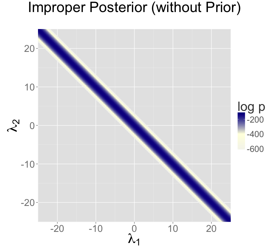
The following plots show the posteriors for two intercept parameterization without prior, two intercept parameterization with standard normal prior, and one intercept reparameterization without prior. For all three cases, the posterior is plotted for 100 data points drawn from a standard normal.

下面的图示展示了没有先验分布的两个截距参数化、具有标准正态先验分布的两个截距参数化以及没有先验分布的一个截距重新参数化的后验分布。对于这三种情况，后验分布是基于从标准正态分布中抽取的100个数据点绘制的。

The two intercept parameterization leads to an improper prior with a ridge extending infinitely to the northwest and southeast.

两个截距参数化导致了一个非正规的先验概率，形成一个从西北向东南无限延伸的岭。

Two intercepts with improper prior

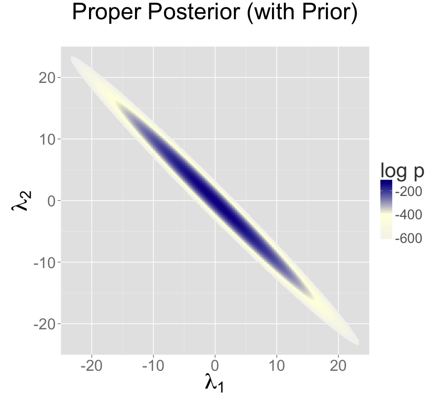
Adding a standard normal prior for the intercepts results in a proper posterior.

通过为截距添加标准正态先验，可以得到一个正规的后验分布。

Two intercepts with proper prior

The single intercept parameterization with no prior also has a proper posterior.

没有先验的单一截距参数化也具有一个正规的后验分布。

Single intercepts with improper prior

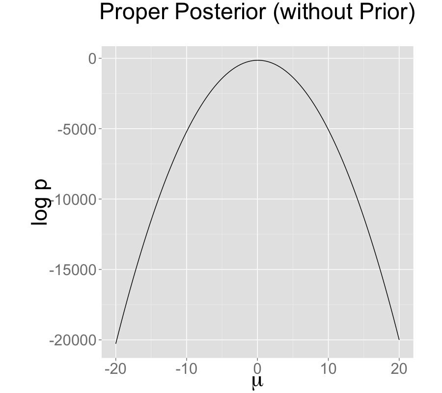
The addition of a prior to the two intercepts model is shown in the second plot; the final plot shows the result of reparameterizing to a single intercept.

在第二张图中展示了对两个截距模型添加先验的结果；最后一张图展示了重新参数化为单个截距的结果。

An alternative strategy for identifying a \(K\)-simplex parameterization \(\theta = \texttt{softmax}(\alpha)\) in terms of an unconstrained \(K\)-vector \(\alpha\) is to place a prior on the components of \(\alpha\) with a fixed location (that is, specifically avoid hierarchical priors with varying location). Unlike the approaching of pinning \(\alpha_K = 0\), the prior-based approach models the \(K\) outcomes symmetrically rather than modeling \(K-1\) outcomes relative to the \(K\)-th. The pinned parameterization, on the other hand, is usually more efficient statistically because it does not have the extra degree of (prior constrained) wiggle room.

另一种识别 \(K\)-单纯形参数化 \(\theta = \texttt{softmax}(\alpha)\) 的策略是在 \(\alpha\) 的各个分量上放置一个具有固定位置的先验概率（特别是避免具有可变位置的分层先验概率）。与将 \(\alpha_K = 0\) 固定不同，基于先验的方法对 \(K\) 个结果进行对称建模，而不是相对于第 \(K\) 个结果对 \(K-1\) 个结果进行建模。另一方面，固定参数化通常在统计上更有效，因为它没有额外的（由先验约束的）自由调整空间。

Vague, strongly informative, and weakly informative priors

模糊先验，强信息先验和弱信息先验

Care must be used when adding a prior to resolve invariances. If the prior is taken to be too broad (i.e., too vague), the resolution is in theory only, and samplers will still struggle.

在添加先验以解决不变性问题时，需要谨慎。如果先验选择过于宽泛（即过于模糊），则解决方案仅在理论上成立，并且采样算法仍然会遇到困难。

Ideally, a realistic prior will be formulated based on substantive knowledge of the problem being modeled. Such a prior can be chosen to have the appropriate strength based on prior knowledge. A strongly informative prior makes sense if there is strong prior information.

理想情况下，应根据对所建模问题的实质性的了解来制定现实的先验概率。这样的先验分布可以根据先前的知识选择适当的强度。如果存在强有力的先验信息，那么选择一个强信息先验是合理的。

When there is not strong prior information, a weakly informative prior strikes the proper balance between controlling computational inference without dominating the data in the posterior. In most problems, the modeler will have at least some notion of the expected scale of the estimates and be able to choose a prior for identification purposes that does not dominate the data, but provides sufficient computational control on the posterior.

当没有强先验信息时，弱信息量的先验概率能够在控制计算推断的同时，不主导后验数据，找到合适的平衡点。在大多数问题中，建模者至少会对估计值的预期范围有一定的了解，并能够选择一个不主导数据但在后验计算上提供足够控制的先验，以达到识别目的。

Priors can also be used in the same way to control the additive invariance of the IRT model. A typical approach is to place a strong prior on student ability parameters \(\alpha\) to control scale simply to control the additive invariance of the basic IRT model and the multiplicative invariance of the model extended with a item discrimination parameters; such a prior does not add any prior knowledge to the problem. Then a prior on item difficulty can be chosen that is either informative or weakly informative based on prior knowledge of the problem.

先验概率也可以用于控制 IRT 模型的加法不变性。一种常见的方法是在学生能力参数 \(\alpha\) 上放置强先验概率，以控制尺度，从而控制基本 IRT 模型的加法不变性，并扩展了项目辨别参数的乘法不变性；这样的先验概率不会为问题增加任何先验知识。然后，可以根据问题的先前知识选择对项目难度的先验概率，这可以是具有信息量或弱信息量的先验。

24.2 Label switching in mixture models

混合模型中的标签交换问题

Where collinearity in regression models can lead to infinitely many posterior maxima, swapping components in a mixture model leads to finitely many posterior maxima.

在回归模型中，共线性可能导致无限多个后验最大值，而在混合模型中，交换成分会导致有限多个后验最大值。

Mixture models

混合模型

Consider a normal mixture model with two location parameters \(\mu_1\) and \(\mu_2\), a shared scale \(\sigma > 0\), a mixture ratio \(\theta \in [0,1]\), and data model

考虑一个带有两个位置参数 \(\mu_1\) 和 \(\mu_2\)、共享尺度 \(\sigma > 0\)、混合比例 \(\theta \in [0,1]\) 的正态混合模型，以及数据模型：

\[ p(y \mid \theta,\mu_1,\mu_2,\sigma) = \prod_{n=1}^N \big( \theta \, \textsf{normal}(y_n \mid \mu_1,\sigma) + (1 - \theta) \, \textsf{normal}(y_n \mid \mu_2,\sigma) \big). \] The issue here is exchangeability of the mixture components, because

这里的问题是混合成分的可交换性，因为

\[ p(\theta,\mu_1,\mu_2,\sigma \mid y) = p\big((1-\theta),\mu_2,\mu_1,\sigma \mid y\big). \] The problem is exacerbated as the number of mixture components \(K\) grows, as in clustering models, leading to \(K!\) identical posterior maxima.

随着混合成分数量 \(K\) 的增加（例如在聚类模型中），这个问题会变得更加严重，导致出现 \(K!\) 个相同的后验最大值。

Convergence monitoring and effective sample size

收敛监测和有效样本量

The analysis of posterior convergence and effective sample size is also difficult for mixture models. For example, the \(\hat{R}\) convergence statistic reported by Stan and the computation of effective sample size are both compromised by label switching. The problem is that the posterior mean, a key ingredient in these computations, is affected by label switching, resulting in a posterior mean for \(\mu_1\) that is equal to that of \(\mu_2\), and a posterior mean for \(\theta\) that is always 1/2, no matter what the data are.

对于混合模型来说，分析后验收敛和有效样本量也是困难的。例如，Stan 报告的 \(\hat{R}\) 收敛统计量和有效样本量的计算都会受到标签切换的影响。问题在于在这些计算中的关键要素后验均值，受到了标签交换的影响，导致 \(\mu_1\) 的后验均值等于 \(\mu_2\) 的后验均值，并且无论数据是什么，\(\theta\) 的后验均值始终为1/2。

Some inferences are invariant

一些推断具有不变性

In some sense, the index (or label) of a mixture component is irrelevant. Posterior predictive inferences can still be carried out without identifying mixture components. For example, the log probability of a new observation does not depend on the identities of the mixture components. The only sound Bayesian inferences in such models are those that are invariant to label switching. Posterior means for the parameters are meaningless because they are not invariant to label switching; for example, the posterior mean for \(\theta\) in the two component mixture model will always be 1/2.

在某种意义上，混合成分的索引（或标签）是无关紧要的。即使不确定混合成分的情况下，后验预测推断仍然可以进行。例如，新观测的对数概率不依赖于混合成分的身份。在这种情况下，唯一可靠的贝叶斯推断是对标签交换具有不变性的推断。参数的后验均值是没有意义的，因为它们对标签交换不具有不变性；例如，在两个成分的混合模型中，\(\theta\) 的后验均值始终为 1/2。

Highly multimodal posteriors

高度多峰后验分布

Theoretically, this should not present a problem for inference because all of the integrals involved in posterior predictive inference will be well behaved. The problem in practice is computation.

理论上，这对推断应该不构成问题，因为后验预测推断中涉及的所有积分都表现良好。实际上的问题在于计算。

Being able to carry out such invariant inferences in practice is an altogether different matter. It is almost always intractable to find even a single posterior mode, much less balance the exploration of the neighborhoods of multiple local maxima according to the probability masses. In Gibbs sampling, it is unlikely for \(\mu_1\) to move to a new mode when sampled conditioned on the current values of \(\mu_2\) and \(\theta\). For HMC and NUTS, the problem is that the sampler gets stuck in one of the two “bowls” around the modes and cannot gather enough energy from random momentum assignment to move from one mode to another.

在实践中能够进行这样的不变推断是一个完全不同的问题。寻找一个后验峰值甚至是平衡对多个局部最大值邻域的探索，根据概率密度进行探索，几乎总是不可行的。在 Gibbs 采样中，当在当前的 \(\mu_2\) 和 \(\theta\) 的值给定的条件下对 \(\mu_1\) 进行采样时，\(\mu_1\) 移动到新峰值的概率是很低的。对于 HMC 和 NUTS，问题在于采样器陷入了围绕模式的两个”碗”之一，并且无法从随机动量分配中获得足够的能量来从一个峰值转移到另一个峰值。

Even with a proper posterior, all known sampling and inference techniques are notoriously ineffective when the number of modes grows super-exponentially as it does for mixture models with increasing numbers of components.

即使选择了一个合适的先验分布,当模型中的成分数量增加时,可能出现的峰值(mode)数量将呈现出超指数级的增长。这会导致所有已知的抽样和推断技术的效果都变得非常糟糕。这个问题在混合模型中表现得尤为突出,因为混合模型通常包含大量的成分。

Hacks as fixes

修复标签交换问题的技巧

Several hacks (i.e., “tricks”) have been suggested and employed to deal with the problems posed by label switching in practice.

在实践中，已经提出并使用了一些技巧来解决标签交换所带来的问题。

Parameter ordering constraints

参数排序约束

One common strategy is to impose a constraint on the parameters that identifies the components. For instance, we might consider constraining \(\mu_1 < \mu_2\) in the two-component normal mixture model discussed above. A problem that can arise from such an approach is when there is substantial probability mass for the opposite ordering \(\mu_1 > \mu_2\). In these cases, the posteriors are affected by the constraint and true posterior uncertainty in \(\mu_1\) and \(\mu_2\) is not captured by the model with the constraint. In addition, standard approaches to posterior inference for event probabilities is compromised. For instance, attempting to use \(M\) posterior samples to estimate \(\Pr[\mu_1 > \mu_2]\), will fail, because the estimator

一种常见的策略是对参数进行约束，以确定各个成分。例如，在上面讨论的两个成分的正态混合模型中，我们可以考虑对参数 \(\mu_1\) 和 \(\mu_2\) 施加约束 \(\mu_1 < \mu_2\)。然而，这种方法可能会引发一个问题，即当相反的顺序 \(\mu_1 > \mu_2\) 具有相当大的概率质量时。在这些情况下,后验分布会受到约束的影响,而 \(\mu_1\) 和 \(\mu_2\) 的真实后验不确定性无法被带约束的模型捕捉到。此外，用于事件概率的后验推断的标准方法也会受到影响。例如，试图使用 \(M\) 个后验样本估计 \(\textsf{Pr}[\mu_1 > \mu_2]\) 将会失败，因为估计量

\[ \Pr[\mu_1 > \mu_2] \approx \sum_{m=1}^M \textrm{I}\left(\mu_1^{(m)} > \mu_2^{(m)}\right) \] will result in an estimate of 0 because the posterior respects the constraint in the model.

将得到一个估计值为0，因为后验符合模型中的约束条件。

Initialization around a single mode

在单个峰周围进行初始化

Another common approach is to run a single chain or to initialize the parameters near realistic values.⁷

另一种常见方法是运行单个马尔可夫链，或将参数初始化在合理的值附近。⁸

This can work better than the hard constraint approach if reasonable initial values can be found and the labels do not switch within a Markov chain. The result is that all chains are glued to a neighborhood of a particular mode in the posterior.

如果能够找到合理的初始值并且标签在马尔可夫链中不会交换，这种方法比硬约束方法更有效。其结果是,所有的马尔可夫链都被”粘住”在后验分布的特定峰值邻域内。

24.3 Component collapsing in mixture models

混合模型中的成分合并

It is possible for two mixture components in a mixture model to collapse to the same values during sampling or optimization. For example, a mixture of \(K\) normals might devolve to have \(\mu_i = \mu_j\) and \(\sigma_i = \sigma_j\) for \(i \neq j\).

在混合模型的采样或优化过程中,有可能出现两个混合成分退化为相同值的情况。例如,在一个包含 \(K\) 个正态分布的混合模型中,可能会出现 \(\mu_i = \mu_j\) 且 \(\sigma_i = \sigma_j\) 的情况,其中 \(i \neq j\)。

This will typically happen early in sampling due to initialization in MCMC or optimization or arise from random movement during MCMC. Once the parameters match for a given draw \((m)\), it can become hard to escape because there can be a trough of low-density mass between the current parameter values and the ones without collapsed components.

这种情况通常会在采样的早期阶段发生,原因可能是 MCMC 或优化算法中的初始化,或者是 MCMC 过程中的随机移动导致的。一旦在某次抽样 \((m)\) 中,两个成分的参数变得相同,就可能变得难以摆脱这种状态,因为在当前参数值与未退化成分的参数值之间,可能存在一个低密度概率质量的”洼地”。

It may help to use a smaller step size during warmup, a stronger prior on each mixture component’s membership responsibility. A more extreme measure is to include additional mixture components to deal with the possibility that some of them may collapse.

在预热阶段使用较小的步长，对每个混合成分的成员责任（membership responsibility）使用更强的先验，可能有助于解决这个问题。一个更极端的措施是增加额外的混合成分，以处理其中一些成分可能退化的情况。

In general, it is difficult to recover exactly the right \(K\) mixture components in a mixture model as \(K\) increases beyond one (yes, even a two-component mixture can have this problem).

一般来说，当 \(K\) 增加到超过1时，在混合模型中精确恢复正确的 \(K\) 个混合成分是困难的（是的，即使是两个成分的混合模型也可能存在此问题）。

24.4 Posteriors with unbounded densities

具有无界密度函数的后验分布

In some cases, the posterior density grows without bounds as parameters approach certain poles or boundaries. In such, there are no posterior modes and numerical stability issues can arise as sampled parameters approach constraint boundaries.

在某些情况下，随着参数接近某些极点或边界，后验密度会无限增长。在这种情况下，不存在后验众数，并且当采样参数接近约束边界时，可能会出现数值稳定性问题。

Mixture models with varying scales

具有变化尺度的混合模型

One such example is a binary mixture model with scales varying by component, \(\sigma_1\) and \(\sigma_2\) for locations \(\mu_1\) and \(\mu_2\). In this situation, the density grows without bound as \(\sigma_1 \rightarrow 0\) and \(\mu_1 \rightarrow y_n\) for some \(n\); that is, one of the mixture components concentrates all of its mass around a single data item \(y_n\).

一个例子是具有不同尺度的二元混合模型，其中各个分量的尺度为 \(\sigma_1\) 和 \(\sigma_2\)，对应于位置参数 \(\mu_1\) 和 \(\mu_2\)。在这种情况下，当 \(\sigma_1 \rightarrow 0\) 且 \(\mu_1 \rightarrow y_n\)（其中 \(n\) 为某个值）时，密度会无限增长；换句话说，其中一个混合成分将其质量集中在单个数据项 \(y_n\) 上。

Beta-binomial models with skewed data and weak priors

具有偏态数据和弱先验的 Beta-binomial 模型

Another example of unbounded densities arises with a posterior such as \(\textsf{beta}(\phi \mid 0.5,0.5)\), which can arise if seemingly weak beta priors are used for groups that have no data. This density is unbounded as \(\phi \rightarrow 0\) and \(\phi \rightarrow 1\). Similarly, a Bernoulli data model coupled with a “weak” beta prior, leads to a posterior

另一个无界密度函数的例子是后验分布 \(\textsf{beta}(\phi \mid 0.5, 0.5)\)，当对没有数据的群体使用看似弱的贝塔先验时，可能会出现这种情况。当 \(\phi \rightarrow 0\) 和 \(\phi \rightarrow 1\) 时，该密度函数是无界的。同样，与”弱”贝塔先验结合的伯努利似然模型会导致后验分布为

\[\begin{align*} p(\phi \mid y) &\propto \textsf{beta}(\phi \mid 0.5,0.5) \times \prod_{n=1}^N \textsf{Bernoulli}(y_n \mid \phi) \\ &= \textsf{beta}\left(\phi \,\middle|\, 0.5 + \sum_{n=1}^N y_n, 0.5 + N - \sum_{n=1}^N y_n\right). \end{align*}\]

If \(N = 9\) and each \(y_n = 1\), the posterior is \(\textsf{beta}(\phi \mid 9.5,0,5)\). This posterior is unbounded as \(\phi \rightarrow 1\). Nevertheless, the posterior is proper, and although there is no posterior mode, the posterior mean is well-defined with a value of exactly 0.95.

如果 \(N = 9\) 且每个 \(y_n = 1\)，后验分布将为 \(\textsf{beta}(\phi \mid 9.5,0.5)\)。当 \(\phi \rightarrow 1\) 时，该后验分布是无界的。尽管没有后验众数（峰值，mode），但后验均值是明确定义的，并且其值恰好为0.95。

Constrained vs. unconstrained scales

受限制与非受限制尺度

Stan does not sample directly on the constrained \((0,1)\) space for this problem, so it doesn’t directly deal with unconstrained density values. Rather, the probability values \(\phi\) are logit-transformed to \((-\infty,\infty)\). The boundaries at 0 and 1 are pushed out to \(-\infty\) and \(\infty\) respectively. The Jacobian adjustment that Stan automatically applies ensures the unconstrained density is proper. The adjustment for the particular case of \((0,1)\) is \(\log \operatorname{logit}^{-1}(\phi) + \log \operatorname{logit}(1 - \phi)\).

在这个问题中，Stan 方法并不直接在受限制的 \((0,1)\) 空间上采样，因此不直接处理非受限制的密度值。相反，概率值 \(\phi\) 经过逻辑(logit)变换转换为 \((-\infty,\infty)\) 空间。0和1处的边界被推到 \(-\infty\) 和 \(\infty\)。Stan 自动应用的 Jacobian 调整确保了非受限制的密度是正规的。对于 \((0,1)\) 的特定情况，调整为 \(\log \operatorname{logit}^{-1}(\phi) + \log \operatorname{logit}(1 - \phi)\)。

There are two problems that still arise, though. The first is that if the posterior mass for \(\phi\) is near one of the boundaries, the logit-transformed parameter will have to sweep out long paths and thus can dominate the U-turn condition imposed by the no-U-turn sampler (NUTS). The second issue is that the inverse transform from the unconstrained space to the constrained space can underflow to 0 or overflow to 1, even when the unconstrained parameter is not infinite. Similar problems arise for the expectation terms in logistic regression, which is why the logit-scale parameterizations of the Bernoulli and binomial distributions are more stable.

然而，仍然存在两个问题。首先，如果 \(\phi\) 的后验质量接近其中一个边界，logit 变换后的参数将需要扫描很长的路径，从而可能主导无转弯条件（no-U-turn sampler, NUTS）所施加的条件。第二个问题是，从非受限制空间到受限制空间的逆变换可能会下溢到0或上溢到1，即使非受限制的参数并非无穷大。类似的问题也会在逻辑回归的期望项中出现，这就是伯努利分布和二项分布的 logit-scale 参数化更稳定的原因。

24.5 Posteriors with unbounded parameters

具有无界参数的后验分布

In some cases, the posterior density will not grow without bound, but parameters will grow without bound with gradually increasing density values. Like the models discussed in the previous section that have densities that grow without bound, such models also have no posterior modes.

在某些情况下，后验密度函数不会无限增长，但参数值会随着密度值的逐渐增加而无限增长。与前一节中讨论的密度函数无限增长的模型类似，这些模型也没有后验峰值。

Separability in logistic regression

逻辑回归中的可分离性

Consider a logistic regression model with \(N\) observed outcomes \(y_n \in \{ 0, 1 \}\), an \(N \times K\) matrix \(x\) of predictors, a \(K\)-dimensional coefficient vector \(\beta\), and data model

考虑一个逻辑回归模型，其中有 \(N\) 个观测结果 \(y_n \in \{0, 1\}\)，一个 \(N \times K\) 的预测变量矩阵 \(x\)，一个 \(K\) 维系数向量 \(\beta\)，以及数据模型

\[ y_n \sim \textsf{Bernoulli}(\operatorname{logit}^{-1}(x_n \beta)). \] Now suppose that column \(k\) of the predictor matrix is such that \(x_{n,k} > 0\) if and only if \(y_n = 1\), a condition known as “separability.” In this case, predictive accuracy on the observed data continue to improve as \(\beta_k \rightarrow \infty\), because for cases with \(y_n = 1\), \(x_n \beta \rightarrow \infty\) and hence \(\operatorname{logit}^{-1}(x_n \beta) \rightarrow 1\).

现在假设预测变量矩阵的第 \(k\) 列满足条件：当且仅当 \(y_n = 1\) 时，\(x_{n,k} > 0\)，这种情况被称为“可分离性”（separability）。在这种情况下，对于观测数据，预测准确性将随着\(\beta_k \rightarrow \infty\) 而持续提高，因为对于 \(y_n = 1\) 的情况，\(x_n \beta \rightarrow \infty\)，从而 \(\operatorname{logit}^{-1}(x_n \beta) \rightarrow 1\)。

With separability, there is no maximum to the likelihood and hence no maximum likelihood estimate. From the Bayesian perspective, the posterior is improper and therefore the marginal posterior mean for \(\beta_k\) is also not defined. The usual solution to this problem in Bayesian models is to include a proper prior for \(\beta\), which ensures a proper posterior.

在可分离性的情况下，似然函数没有最大值，因此也没有最大似然估计。从贝叶斯的角度来看，后验分布是不合适的，因此 \(\beta_k\) 的边际后验均值也没有定义。在贝叶斯模型中解决这个问题的通常方法是为 \(\beta\) 引入一个正规的先验分布，以确保有正规的后验分布。

24.6 Uniform posteriors

均匀后验分布

Suppose your model includes a parameter \(\psi\) that is defined on \([0,1]\) and is given a flat prior \(\textsf{uniform}(\psi \mid 0,1)\). Now if the data don’t tell us anything about \(\psi\), the posterior is also \(\textsf{uniform}(\psi \mid 0,1)\).

假设你的模型包含一个参数 \(\psi\)，其取值范围为 \([0,1]\)，并且给定了一个均匀先验分布 \(\textsf{uniform}(\psi \mid 0,1)\)。如果数据对 \(\psi\) 没有提供任何信息，那么后验分布也将是 \(\textsf{uniform}(\psi \mid 0,1)\)。

Although there is no maximum likelihood estimate for \(\psi\), the posterior is uniform over a closed interval and hence proper. In the case of a uniform posterior on \([0,1]\), the posterior mean for \(\psi\) is well-defined with value \(1/2\). Although there is no posterior mode, posterior predictive inference may nevertheless do the right thing by simply integrating (i.e., averaging) over the predictions for \(\psi\) at all points in \([0,1]\).

尽管对于 \(\psi\) 没有最大似然估计值，但后验分布在闭区间上是均匀的，因此是正规的。在后验均匀分布在 \([0,1]\) 的情况下，\(\psi\) 的后验均值是有定义的，其值为 \(1/2\)。尽管没有后验模式，但通过对 \([0, 1]\) 中所有点的 \(\psi\) 的预测进行积分（平均），后验预测推断仍然可以得到正确的结果。

24.7 Sampling difficulties with problematic priors

具有问题先验的抽样的困难

With an improper posterior, it is theoretically impossible to properly explore the posterior. However, Gibbs sampling as performed by BUGS and JAGS, although still unable to properly sample from such an improper posterior, behaves differently in practice than the Hamiltonian Monte Carlo sampling performed by Stan when faced with an example such as the two intercept model discussed in the collinearity section and illustrated in the non-identifiable density plot.

对于非正规的后验分布，理论上是不可能进行正确的探索后验分布的。然而，BUGS 和 JAGS 等进行的 Gibbs 抽样在实践中与 Stan 进行的 Hamiltonian Monte Carlo (HMC)抽样在面对多重共线性部分中讨论的双截距模型时表现不同，这也在非可辨识密度图中进行了说明。

Gibbs sampling

Gibbs 抽样

Gibbs sampling, as performed by BUGS and JAGS, may appear to be efficient and well behaved for this unidentified model, but as discussed in the previous subsection, will not actually explore the posterior properly.

BUGS 和 JAGS 等软件实现的 Gibbs 抽样可能在处理该不可辨识模型时表现出高效和良好的行为，但正如前面的子节中讨论的那样，它实际上无法正确地探索后验分布。虽然 Gibbs 抽样在表面上看起来效果良好，但它并不能提供对后验分布的准确估计。

Consider what happens with initial values \(\lambda_1^{(0)}, \lambda_2^{(0)}\). Gibbs sampling proceeds in iteration \(m\) by drawing

考虑初始值\(\lambda_1^{(0)}, \lambda_2^{(0)}\)。在 Gibbs 抽样中，通过迭代进行抽样。对于第 \(m\) 次迭代，我们从以下条件分布中抽取新的参数值：

\[\begin{align*} \lambda_1^{(m)} &\sim p(\lambda_1 \mid \lambda_2^{(m-1)}, \sigma^{(m-1)}, y) \\ \lambda_2^{(m)} &\sim p(\lambda_2 \mid \lambda_1^{(m)}, \sigma^{(m-1)}, y) \\ \sigma^{(m)} &\sim p(\sigma \mid \lambda_1^{(m)}, \lambda_2^{(m)}, y). \end{align*}\]

Now consider the draw for \(\lambda_1\) (the draw for \(\lambda_2\) is symmetric), which is conjugate in this model and thus can be done efficiently. In this model, the range from which the next \(\lambda_1\) can be drawn is highly constrained by the current values of \(\lambda_2\) and \(\sigma\). Gibbs will run quickly and provide seemingly reasonable inferences for \(\lambda_1 + \lambda_2\). But it will not explore the full range of the posterior; it will merely take a slow random walk from the initial values. This random walk behavior is typical of Gibbs sampling when posteriors are highly correlated and the primary reason to prefer Hamiltonian Monte Carlo to Gibbs sampling for models with parameters correlated in the posterior.

现在考虑对 \(\lambda\_1\) 的抽样（对 \(\lambda\_2\) 的抽样与此对称），在这个模型中，由于采用了共轭先验，这一步抽样可以高效完成。然而，在实际操作中，下一个 \(\lambda\_1\) 的取值范围受到当前 \(\lambda\_2\) 和 \(\sigma\) 值的高度约束。虽然 Gibbs 抽样能快速运行，并为 \(\lambda\_1 + \lambda\_2\) 提供看似合理的推断结果，但实际上它并未充分探索后验分布的整个范围，而仅仅从初始值附近缓慢地进行随机漫步。这种随机漫步的特征在后验相关性较高的情形下尤为明显，也是为何在参数后验分布存在高度相关性时，更倾向于使用 Hamiltonian Monte Carlo 而非 Gibbs 抽样的重要原因之一。

Hamiltonian Monte Carlo sampling

Hamiltonian Monte Carlo 抽样

Hamiltonian Monte Carlo (HMC), as performed by Stan, is much more efficient at exploring posteriors in models where parameters are correlated in the posterior. In this particular example, the Hamiltonian dynamics (i.e., the motion of a fictitious particle given random momentum in the field defined by the negative log posterior) is going to run up and down along the valley defined by the potential energy (ridges in log posteriors correspond to valleys in potential energy). In practice, even with a random momentum for \(\lambda_1\) and \(\lambda_2\), the gradient of the log posterior is going to adjust for the correlation and the simulation will run \(\lambda_1\) and \(\lambda_2\) in opposite directions along the valley corresponding to the ridge in the posterior log density.

Stan 执行的 Hamiltonian Monte Carlo (HMC)在探索参数后验分布中具有相关性的模型中更加高效。在这个特定的例子中，Hamiltonian 动力学（即，在由负对数后验定义的场中，给予虚拟粒子随机动量后的运动）将沿着由势能定义的山谷上下运行（log 后验中的岭对应势能中的山谷）。实际上，即使对于 \(\lambda_1\) 和 \(\lambda_2\) 随机给定动量，对数后验的梯度也会调整以适应它们之间的相关性，从而使得模拟中的 \(\lambda_1\) 和 \(\lambda_2\) 沿着对应于后验密度中岭的山谷相反的方向运行。

No-U-turn sampling

No-U-turn 抽样

Stan’s default no-U-turn sampler (NUTS), is even more efficient at exploring the posterior (see Hoffman and Gelman 2014). NUTS simulates the motion of the fictitious particle representing the parameter values until it makes a U-turn, it will be defeated in most cases, as it will just move down the potential energy valley indefinitely without making a U-turn. What happens in practice is that the maximum number of leapfrog steps in the simulation will be hit in many of the iterations, causing a large number of log probability and gradient evaluations (1000 if the max tree depth is set to 10, as in the default). Thus sampling will appear to be slow. This is indicative of an improper posterior, not a bug in the NUTS algorithm or its implementation. It is simply not possible to sample from an improper posterior! Thus the behavior of HMC in general and NUTS in particular should be reassuring in that it will clearly fail in cases of improper posteriors, resulting in a clean diagnostic of sweeping out large paths in the posterior.

Stan 默认的 no-U-turn 抽样器（NUTS）在探索后验分布方面更加高效[参见@Hoffman-Gelman:2014]。NUTS 模拟了代表参数值的虚拟粒子的运动，直到它产生一个 U-turn。然而，在大多数情况下，NUTS 会失败，因为它将无限期地沿着势能山谷向下移动，而不会产生 U-turn。实际情况是,在许多迭代中,会达到模拟的最大”跳跃步”数，导致大量的对数概率和梯度计算（默认情况下，如果将最大树深度设置为10，则有1000个计算）。因此，采样看起来会很慢。这表明后验分布是不适当的，而不是 NUTS 算法或其实现存在问题。从不适当的后验分布中进行采样是不可能的！因此，HMC 的行为一般而言，尤其是 NUTS，应该是令人放心的，因为在后验不合适的情况下，它们会明显失效,这能给出清晰的诊断,即后验分布中存在较大范围的异常区域。

Here are results of Stan runs with default parameters fit to \(N=100\) data points generated from \(y_n \sim \textsf{normal}(0,1)\):

以下是使用默认参数拟合生成的 \(N=100\) 个数据点 \(y_n \sim \textsf{normal}(0,1)\) 的 Stan 运行结果：

Two Scale Parameters, Improper Prior

两个规模参数，非正规的先验

Inference for Stan model: improper_stan
Warmup took (2.7, 2.6, 2.9, 2.9) seconds, 11 seconds total
Sampling took (3.4, 3.7, 3.6, 3.4) seconds, 14 seconds total

                  Mean     MCSE   StdDev        5%       95%  N_Eff  N_Eff/s  R_hat
lp__          -5.3e+01  7.0e-02  8.5e-01  -5.5e+01  -5.3e+01    150       11    1.0
n_leapfrog__   1.4e+03  1.7e+01  9.2e+02   3.0e+00   2.0e+03   2987      212    1.0
lambda1        1.3e+03  1.9e+03  2.7e+03  -2.3e+03   6.0e+03    2.1     0.15    5.2
lambda2       -1.3e+03  1.9e+03  2.7e+03  -6.0e+03   2.3e+03    2.1     0.15    5.2
sigma          1.0e+00  8.5e-03  6.2e-02   9.5e-01   1.2e+00     54      3.9    1.1
mu             1.6e-01  1.9e-03  1.0e-01  -8.3e-03   3.3e-01   2966      211    1.0

Two Scale Parameters, Weak Prior

两个规模参数，较弱的先验

Warmup took (0.40, 0.44, 0.40, 0.36) seconds, 1.6 seconds total
Sampling took (0.47, 0.40, 0.47, 0.39) seconds, 1.7 seconds total

                 Mean     MCSE   StdDev        5%    95%  N_Eff  N_Eff/s  R_hat
lp__              -54  4.9e-02  1.3e+00  -5.7e+01    -53    728      421    1.0
n_leapfrog__      157  2.8e+00  1.5e+02   3.0e+00    511   3085     1784    1.0
lambda1          0.31  2.8e-01  7.1e+00  -1.2e+01     12    638      369    1.0
lambda2         -0.14  2.8e-01  7.1e+00  -1.2e+01     12    638      369    1.0
sigma             1.0  2.6e-03  8.0e-02   9.2e-01    1.2    939      543    1.0
mu               0.16  1.8e-03  1.0e-01  -8.1e-03   0.33   3289     1902    1.0

One Scale Parameter, Improper Prior

一个规模参数，非正规的先验

Warmup took (0.011, 0.012, 0.011, 0.011) seconds, 0.044 seconds total
Sampling took (0.017, 0.020, 0.020, 0.019) seconds, 0.077 seconds total

预热阶段耗时(0.011, 0.012, 0.011, 0.011)秒，总计0.044秒
抽样阶段耗时(0.017, 0.020, 0.020, 0.019)秒，总计0.077秒

                Mean     MCSE  StdDev        5%   50%   95%  N_Eff  N_Eff/s  R_hat
lp__             -54  2.5e-02    0.91  -5.5e+01   -53   -53   1318    17198    1.0
n_leapfrog__     3.2  2.7e-01     1.7   1.0e+00   3.0   7.0     39      507    1.0
mu              0.17  2.1e-03    0.10  -3.8e-03  0.17  0.33   2408    31417    1.0
sigma            1.0  1.6e-03   0.071   9.3e-01   1.0   1.2   2094    27321    1.0

On the top is the non-identified model with improper uniform priors and data model \(y_n \sim \textsf{normal}(\lambda_1 + \lambda_2, \sigma)\).

第一个是一个具有非正规的均匀先验和似然函数 \(y_n \sim \textsf{normal}(\lambda_1 + \lambda_2, \sigma)\) 的不可识别模型。

In the middle is the same data model as in top plus priors \(\lambda_k \sim \textsf{normal}(0,10)\).

在中间的模型中，与上述模型相同的数据模型结合了先验分布 \(\lambda_k \sim \textsf{normal}(0,10)\)。

On the bottom is an identified model with an improper prior, with data model \(y_n \sim \textsf{normal}(\mu,\sigma)\). All models estimate \(\mu\) at roughly 0.16 with low Monte Carlo standard error, but a high posterior standard deviation of 0.1; the true value \(\mu=0\) is within the 90% posterior intervals in all three models.

最后一个是一个具有非正规的先验、似然函数 \(y_n \sim \textsf{normal}(\mu,\sigma)\) 的可识别模型。所有模型对 \(\mu\) 的估计大致在0.16左右，具有较低的蒙特卡洛标准误差，但后验标准差较高，为 0.1；真实值 \(\mu=0\) 在这三个模型的90%后验区间内。

Examples: fits in Stan

例子：在 stan 中拟合

To illustrate the issues with sampling from non-identified and only weakly identified models, we fit three models with increasing degrees of identification of their parameters. The posteriors for these models is illustrated in the non-identifiable density plot. The first model is the unidentified model with two location parameters and no priors discussed in the collinearity section.

为了说明从非可识别模型和仅具有弱标识的模型中采样的问题，我们拟合了三个模型，其参数的可识别程度逐渐增加。这些模型的后验分布在非可识别密度图中进行了说明。第一个模型是在collinearity section中讨论的具有两个位置参数且没有先验分布的不可识别模型。

data {
  int N;
  array[N] real y;
}
parameters {
  real lambda1;
  real lambda2;
  real<lower=0> sigma;
}
transformed parameters {
  real mu;
  mu = lambda1 + lambda2;
}
model {
  y ~ normal(mu, sigma);
}

The second adds priors to the model block for lambda1 and lambda2 to the previous model.

第二个模型在前一个模型的基础上，在模型块中为 lambda1 和 lambda2 添加了先验分布。

lambda1 ~ normal(0, 10);
lambda2 ~ normal(0, 10);

The third involves a single location parameter, but no priors.

第三个模型只涉及一个位置参数，没有使用先验分布。

data {
  int N;
  array[N] real y;
}
parameters {
  real mu;
  real<lower=0> sigma;
}
model {
  y ~ normal(mu, sigma);
}

All three of the example models were fit in Stan 2.1.0 with default parameters (1000 warmup iterations, 1000 sampling iterations, NUTS sampler with max tree depth of 10). The results are shown in the non-identified fits figure. The key statistics from these outputs are the following.

这三个示例模型均使用 Stan 2.1.0的默认参数进行拟合（1000个预热迭代、1000个抽样迭代，NUTS 采样器，最大树深度为10）。结果显示在非可识别拟合图中。这些输出的关键统计数据如下所示。

• As indicated by R_hat column, all parameters have converged other than \(\lambda_1\) and \(\lambda_2\) in the non-identified model.

• 如R_hat列所示，除了非可辨识模型中的 \(\lambda_1\) 和 \(\lambda_2\) 之外，所有参数都已收敛。

• The average number of leapfrog steps is roughly 3 in the identified model, 150 in the model identified by a weak prior, and 1400 in the non-identified model.

• 在可辨识模型中，平均跳跃步数大约为3步；在通过弱先验得到可辨识的模型中，平均跳跃步数为150步；而在非可辨识模型中，平均跳跃步数为1400步。

• The number of effective samples per second for \(\mu\) is roughly 31,000 in the identified model, 1,900 in the model identified with weakly informative priors, and 200 in the non-identified model; the results are similar for \(\sigma\).

• 在可辨识模型中，\(\mu\) 的每秒有效样本数大约为31,000个；在通过弱信息先验得到可辨识的模型中，每秒有效样本数为1,900个；而在非可辨识模型中，每秒有效样本数为200个。\(\sigma\) 的结果类似。

• In the non-identified model, the 95% interval for \(\lambda_1\) is (-2300,6000), whereas it is only (-12,12) in the model identified with weakly informative priors.

• 在非可辨识模型中，\(\lambda_1\) 的95%置信区间为(-2300,6000)，而在通过弱信息先验得到可辨识的模型中，该置信区间仅为(-12, 12)。

• In all three models, the simulated value of \(\mu=0\) and \(\sigma=1\) are well within the posterior 90% intervals.

• 在所有三个模型中，模拟得到的 \(\mu=0\) 和 \(\sigma=1\) 都在后验的90%置信区间内。

The first two points, lack of convergence and hitting the maximum number of leapfrog steps (equivalently maximum tree depth) are indicative of improper posteriors. Thus rather than covering up the problem with poor sampling as may be done with Gibbs samplers, Hamiltonian Monte Carlo tries to explore the posterior and its failure is a clear indication that something is amiss in the model.

前两点，收敛不足和达到最大的跃点步数（等价于最大的树深度）都表明后验分布是非正规的。与 Gibbs 采样器可能通过低质量采样来掩盖问题的情况不同，Hamiltonian Monte Carlo 试图探索后验分布，而其失败清楚地表明了模型存在问题。

Hoffman, Matthew D., and Andrew Gelman. 2014. “The No-U-Turn Sampler: Adaptively Setting Path Lengths in Hamiltonian Monte Carlo.” Journal of Machine Learning Research 15: 1593–623. http://jmlr.org/papers/v15/hoffman14a.html.

Neal, Radford M. 1996. “Sampling from Multimodal Distributions Using Tempered Transitions.” Statistics and Computing 6 (4): 353–66.

Swendsen, Robert H., and Jian-Sheng Wang. 1986. “Replica Monte Carlo Simulation of Spin Glasses.” Physical Review Letters 57: 2607–9.

---

1. This example was raised by Richard McElreath on the Stan users group in a query about the difference in behavior between Gibbs sampling as used in BUGS and JAGS and the Hamiltonian Monte Carlo (HMC) and no-U-turn samplers (NUTS) used by Stan.

2. 这个例子是 Richard McElreath 在 Stan 用户组中提出的,他询问了 BUGS 和 JAGS 中使用的 Gibbs 采样与 Stan 使用的 Hamiltonian Monte Carlo (HMC)和 no-U-turn 采样器 (NUTS)之间的行为差异。

3. The marginal posterior \(p(\sigma \mid y)\) for \(\sigma\) is proper here as long as there are at least two distinct data points.

4. 只要至少存在两个不同的数据点，那么这里的边际后验分布 \(p(\sigma \mid y)\) 对于 \(\sigma\) 是正规的。

5. A Laplace prior (or an L1 regularizer for penalized maximum likelihood estimation) is not sufficient to remove this additive invariance. It provides shrinkage, but does not in and of itself identify the parameters because adding a constant to \(\lambda_1\) and subtracting it from \(\lambda_2\) results in the same value for the prior density.

6. 一个拉普拉斯先验（或者 L1 正则项用于惩罚最大似然估计）并不足以消除这种加法不变性。它可以提供收缩效果，但本身并不能识别参数，因为在 \(\lambda_1\) 上加上一个常数并从 \(\lambda_2\) 上减去该常数会得到相同的先验密度值。

7. Tempering methods may be viewed as automated ways to carry out such a search for modes, though most MCMC tempering methods continue to search for modes on an ongoing basis; see (Swendsen and Wang 1986; Neal 1996).

8. 退火方法可以视为自动执行此类模式搜索的方法，尽管大多数 MCMC 退火方法仍在不断进行模式搜索；详见 (Swendsen and Wang 1986; Neal 1996).