30 基于模拟的校准
Simulation-Based Calibration
本节译者:郭鑫
初次校审:李君竹
二次校审:李君竹(Claude 辅助)
A Bayesian posterior is calibrated if the posterior intervals have appropriate coverage. For example, 80% intervals are expected to contain the true parameter 80% of the time. If data is generated according to a model, Bayesian posterior inference with respect to that model is calibrated by construction. Simulation-based calibration (SBC) exploits this property of Bayesian inference to assess the soundness of a posterior sampler. Roughly, the way it works is by simulating parameters according to the prior, then simulating data conditioned on the simulated parameters, then testing posterior calibration of the inference algorithm over independently simulated data sets. This chapter follows Talts et al. (2018), which improves on the original approach developed by Cook, Gelman, and Rubin (2006).
如果贝叶斯后验区间具有适当的覆盖率,则称该贝叶斯后验是校准的。例如,80% 的区间预期在 80% 的时间内包含真实参数。如果数据是根据模型生成的,那么基于该模型的贝叶斯后验推断天然就是校准的。基于模拟的校准(Simulation-based calibration,SBC)利用贝叶斯推断的这一特性来评估后验采样器的合理性。大体而言,其工作原理是根据先验模拟参数,然后基于模拟的参数生成数据,再通过独立模拟的数据集测试推断算法的后验校准。本章遵循 Talts et al. (2018),该文改进了 Cook, Gelman, and Rubin (2006) 开发的原始方法。
30.1 Bayes is calibrated by construction
贝叶斯天然具有校准性
Suppose a Bayesian model is given in the form of a prior density \(p(\theta)\) and sampling density \(p(y \mid \theta).\) Now consider a process that first simulates parameters from the prior,
假设贝叶斯模型由先验密度 \(p(\theta)\) 和抽样密度 \(p(y \mid \theta)\) 组成。现在考虑一个过程,首先从先验中模拟参数,
\[ \theta^{\textrm{sim}} \sim p(\theta), \] and then simulates data given the parameters,
然后基于参数模拟数据,
\[ y^{\textrm{sim}} \sim p(y \mid \theta^{\textrm{sim}}). \] By the definition of conditional densities, the simulated data and parameters constitute an independent draw from the model’s joint distribution,
根据条件密度的定义,模拟的数据和参数构成了模型联合分布的独立采样点,
\[ (y^{\textrm{sim}}, \theta^{\textrm{sim}}) \sim p(y, \theta). \] From Bayes’s rule, it follows that for any observed (fixed) data \(y\),
根据贝叶斯定理,对于任何观测到的(固定的)数据 \(y\),
\[ p(\theta \mid y) \propto p(y, \theta). \] Therefore, the simulated parameters constitute a draw from the posterior for the simulated data,
因此,模拟的参数构成了基于模拟数据的后验采样点,
\[ \theta^{\textrm{sim}} \sim p(\theta \mid y^{\textrm{sim}}). \] Now consider an algorithm that produces a sequence of draws from the posterior given this simulated data,
现在考虑一种算法,基于这些模拟数据产生一系列后验采样点,
\[ \theta^{(1)}, \ldots, \theta^{(M)} \sim p(\theta \mid y^{\textrm{sim}}). \] Because \(\theta^{\textrm{sim}}\) is also distributed as a draw from the posterior, the rank statistics of \(\theta^{\textrm{sim}}\) with respect to \(\theta^{(1)}, \ldots \theta^{(M)}\) should be uniform.
因为 \(\theta^{\textrm{sim}}\) 也服从后验分布,所以 \(\theta^{\textrm{sim}}\) 相对于采样点 \(\theta^{(1)}, \ldots \theta^{(M)}\) 的秩统计量应服从均匀分布。
This is one way to define calibration, because it follows that posterior intervals will have appropriate coverage (Dawid 1982; Gneiting, Balabdaoui, and Raftery 2007). If the rank of \(\theta^{\textrm{sim}}\) is uniform among the draws \(\theta^{(1)}, \ldots, \theta^{(M)},\) then for any 90% interval selected, the probability the true value \(\theta^{\textrm{sim}}\) falls in it will also be 90%. The same goes for any other posterior interval.
这是定义校准的一种方式,因为由此可得后验区间将具有适当的覆盖率 (Dawid 1982; Gneiting, Balabdaoui, and Raftery 2007)。如果 \(\theta^{\textrm{sim}}\) 的秩在采样点 \(\theta^{(1)}, \ldots, \theta^{(M)}\) 中服从均匀分布,那么对于任何选定的 90% 区间,真实值 \(\theta^{\textrm{sim}}\) 落在其中的概率也是 90%。其他任何后验区间也是如此。
30.2 Simulation-based calibration
基于模拟的校准
Suppose the Bayesian model to test has joint density
假设要测试的贝叶斯模型具有联合密度
\[ p(y, \theta) = p(y \mid \theta) \cdot p(\theta), \] with data \(y\) and parameters \(\theta\) (both are typically multivariate). Simulation-based calibration works by generating \(N\) simulated parameter and data pairs according to the joint density,
其中数据 \(y\) 和参数 \(\theta\)(两者通常都是多元的)。基于模拟的校准通过根据联合密度生成 \(N\) 个模拟的参数和数据对来工作,
\[ (y^{\textrm{sim}(1)}, \theta^{\textrm{sim}(1)}), \ldots, (y^{\textrm{sim}(N)}, \theta^{\textrm{sim}(N)}), \sim p(y, \theta). \] For each simulated data set \(y^{\textrm{sim}(n)}\), use the algorithm to be tested to generate \(M\) posterior draws, which if everything is working properly, will be distributed marginally as
对于每个模拟数据集 \(y^{\textrm{sim}(n)}\),使用待测试的算法生成 \(M\) 个后验采样点,如果一切正常,它们的边际分布为
\[ \theta^{(n, 1)}, \ldots, \theta^{(n, M)} \sim p(\theta \mid y^{\textrm{sim}(n)}). \] For a simulation \(n\) and parameter \(k\), the rank of the simulated parameter among the posterior draws is
对于模拟 \(n\) 和参数 \(k\),模拟参数在后验采样点中的秩为
\[\begin{eqnarray*} r_{n, k} & = & \textrm{rank}(\theta_k^{\textrm{sim}(n)}, (\theta^{(n, 1)}, \ldots, \theta^{(n,M)})) \\[4pt] & = & \sum_{m = 1}^M \textrm{I}[\theta_k^{(n,m)} < \theta_k^{\textrm{sim}(n)}]. \end{eqnarray*}\] That is, the rank is the number of posterior draws \(\theta^{(n,m)}_k\) that are less than the simulated draw \(\theta^{\textrm{sim}(n)}_k.\)
也就是说,秩是小于模拟值 \(\theta^{\textrm{sim}(n)}_k\) 的后验采样点 \(\theta^{(n,m)}_k\) 的数量。
If the algorithm generates posterior draws according to the posterior, the ranks should be uniformly distributed from \(0\) to \(M\), so that the ranks plus one are uniformly distributed from \(1\) to \(M + 1\),
如果算法根据后验生成后验采样点,则秩应该从 \(0\) 到 \(M\) 均匀分布,因此秩加一从 \(1\) 到 \(M + 1\) 均匀分布,
\[ r_{n, k} + 1 \sim \textrm{categorical}\! \left(\frac{1}{M + 1}, \ldots, \frac{1}{M + 1}\right). \] Simulation-based calibration uses this expected behavior to test the calibration of each parameter of a model on simulated data. Talts et al. (2018) suggest plotting binned counts of \(r_{1:N, k}\) for different parameters \(k\); Cook, Gelman, and Rubin (2006) automate the process with a hypothesis test for uniformity.
基于模拟的校准利用这种预期行为来测试模型各参数在模拟数据上的校准情况。Talts et al. (2018) 建议绘制不同参数 \(k\) 的 \(r_{1:N,k}\) 的分箱计数图;Cook, Gelman, and Rubin (2006) 通过均匀性假设检验实现了该过程的自动化。
30.3 SBC in Stan
Stan 中的 SBC
Running simulation-based calibration in Stan will test whether Stan’s sampling algorithm can sample from the posterior associated with data generated according to the model. The data simulation and posterior fitting and rank calculation can all be done within a single Stan program. Then Stan’s posterior sampler has to be run multiple times. Each run produces a rank for each parameter being assessed for uniformity. The total set of ranks can then be tested for uniformity.
在 Stan 中运行基于模拟的校准将测试 Stan 的采样算法能否从根据模型生成的数据所对应的后验中进行采样。数据模拟、后验拟合和秩计算都可以在单个 Stan 程序中完成。然后需要多次运行 Stan 的后验采样器。每次运行都会为每个待评估均匀性的参数产生一个秩。然后可以测试整个秩集合的均匀性。
Example model
示例模型
For illustration, a very simple model will suffice. Suppose there are two parameters \((\mu, \sigma)\) with independent priors,
为了说明,一个非常简单的模型就足够了。假设有两个参数 \((\mu, \sigma)\) 具有独立的先验,
\[ \mu \sim \textrm{normal}(0, 1), \] and
和
\[ \sigma \sim \textrm{lognormal}(0, 1). \] The data \(y = y_1, \ldots, y_N\) is drawn conditionally independently given the parameters,
数据 \(y = y_1, \ldots, y_N\) 在给定参数的条件下独立抽取,
\[ y_n \sim \textrm{normal}(\mu, \sigma). \] The joint prior density is thus
因此联合先验密度为
\[ p(\mu, \sigma) = \textrm{normal}(\mu \mid 0, 1) \cdot \textrm{lognormal}(\sigma \mid 0, 1), \] and the sampling density is
采样密度为
\[ p(y \mid \mu, \sigma) = \prod_{n=1}^N \textrm{normal}(y_n \mid \mu, \sigma). \]
For example, suppose the following two parameter values are drawn from the prior in the first simulation,
例如,假设在第一次模拟中从先验中抽取了以下两个参数值,
\[ (\mu^{\textrm{sim(1)}}, \sigma^{\textrm{sim(1)}}) = (1.01, 0.23). \] Then data \(y^{\textrm{sim}(1)} \sim p(y \mid \mu^{\textrm{sim(1)}}, \sigma^{\textrm{sim(1)}})\) is drawn according to the sampling distribution. Next, \(M = 4\) draws are taken from the posterior \(\mu^{(1,m)}, \sigma^{(1,m)} \sim p(\mu, \sigma \mid y^{\textrm{sim}(1)})\),
然后根据抽样分布抽取数据 \(y^{\textrm{sim}(1)} \sim p(y \mid \mu^{\textrm{sim(1)}}, \sigma^{\textrm{sim(1)}})\)。接下来,从后验 \(\mu^{(1,m)}, \sigma^{(1,m)} \sim p(\mu, \sigma \mid y^{\textrm{sim}(1)})\) 中抽取 \(M = 4\) 个采样点,
\[ \begin{array}{r|rr} m & \mu^{(1,m)} & \sigma^{(1,m)} \\ \hline 1 & 1.07 & 0.33 \\ 2 & -0.32 & 0.14 \\ 3 & -0.99 & 0.26 \\ 4 & 1.51 & 0.31 \end{array} \] Then the comparisons on which ranks are based look as follows,
然后基于秩的比较如下所示,
\[ \begin{array}{r|cc} m & \textrm{I}(\mu^{(1,m)} < \mu^{\textrm{sim}(1)}) & \textrm{I}(\sigma^{(1,m)} < \sigma^{\textrm{sim}(1)}) \\ \hline 1 & 0 & 0 \\ 2 & 1 & 1 \\ 3 & 1 & 0 \\ 4 & 0 & 0 \end{array} \] The ranks are the column sums, \(r_{1,1} = 2\) and \(r_{1,2} = 1\). Because the simulated parameters are distributed according to the posterior, these ranks should be distributed uniformly between \(0\) and \(M\), the number of posterior draws.
秩是列和,\(r_{1,1} = 2\) 和 \(r_{1,2} = 1\)。因为模拟参数是根据后验分布的,这些秩应该在 \(0\) 和 \(M\)(后验采样点的数量)之间均匀分布。
Testing a Stan program with simulation-based calibration
使用基于模拟的校准测试 Stan 程序
To code simulation-based calibration in a Stan program, the transformed data block can be used to simulate parameters and data from the model. The parameters, transformed parameters, and model block then define the model over the simulated data. Then, in the generated quantities block, the program records an indicator for whether each parameter is less than the simulated value. As shown above, the rank is then the sum of the simulated indicator variables.
要在 Stan 程序中编码基于模拟的校准,可以使用 transformed data 块从模型中模拟参数和数据。然后,parameters、transformed parameters 和 model 块在模拟数据上定义模型。然后,在 generated quantities 块中,程序记录每个参数是否小于模拟值的指示器。如上所示,秩就是模拟指示变量的总和。
transformed data {
  real mu_sim = normal_rng(0, 1);
  real<lower=0> sigma_sim = lognormal_rng(0, 1);
  int<lower=0> J = 10;
  vector[J] y_sim;
  for (j in 1:J) {
    y_sim[j] = normal_rng(mu_sim, sigma_sim);
  }
}
parameters {
  real mu;
  real<lower=0> sigma;
}
model {
  mu ~ normal(0, 1);
  sigma ~ lognormal(0, 1);
  y_sim ~ normal(mu, sigma);
}
generated quantities {
  array[2] int<lower=0, upper=1> lt_sim
      = { mu < mu_sim, sigma < sigma_sim };
}
To avoid confusion with the number of simulated data sets used for simulation-based calibration, J is used for the number of simulated data points.
为了避免与用于基于模拟的校准的模拟数据集数量混淆,J 用于表示模拟数据点的数量。
The model is implemented twice—once as a data generating process using random number generators in the transformed data block, then again in the parameters and model block. This duplication is a blessing and a curse. The curse is that it’s more work and twice the chance for errors. The blessing is that by implementing the model twice and comparing results, the chance of there being a mistake in the model is reduced.
该模型实现了两次——一次作为数据生成过程在 transformed data 块中使用随机数生成器,然后在 parameters 和 model 块中再次实现。这种重复既有利也有弊。弊的是工作量更多,出错的可能性加倍。利的是,通过两次实现模型并比较结果,可以减少模型中出错的可能性。
Pseudocode for simulation-based calibration
基于模拟的校准的伪代码
The entire simulation-based calibration process is as follows, where
整个基于模拟的校准过程如下,其中
p(theta)is the prior densityp(theta)是先验密度p(y | theta)is the sampling densityp(y | theta)是抽样密度Kis the number of parametersK是参数的数量Nis the total number of simulated data sets and fitsN是模拟数据集和拟合的总数Mis the number of posterior draws per simulated data setM是每个模拟数据集的后验采样点数
SBC(p(theta), p(y | theta), K, N, M)
------------------------------------
for (n in 1:N) {
    // simulate parameters and data
    theta(sim(n)) ~ p(theta)
    y(sim(n)) ~ p(y | theta(sim(n)))

    // posterior draws given simulated data
    for (m in 1:M) {
        theta(n, m) ~ p(theta | y(sim(n)))
    }
    // calculate rank of sim among posterior draws
    for (k in 1:K) {
        rank(n, k) = SUM_m I(theta[k](n,m) < theta[k](sim(n)))
    }
}
// test uniformity of each parameter
for (k in 1:K) {
    test uniformity of rank(1:N, k)
}
The importance of thinning
抽稀的重要性
The draws from the posterior are assumed to be roughly independent. If they are not, artifacts may arise in the uniformity tests due to correlation in the posterior draws. Thus it is best to thin the posterior draws down to the point where the effective sample size is roughly the same as the number of thinned draws. This may require running the code a few times to judge the number of draws required to produce a target effective sample size. This operation that can be put into a loop that doubles the number of iterations until all parameters have an effective sample size of M, then thinning down to M draws.
假设来自后验的采样点大致是独立的。如果不是,由于后验采样点中的相关性,均匀性测试中可能会出现伪影。因此,最好将后验采样点抽稀到有效样本量与抽稀后采样点数大致相同的程度。这可能需要运行几次代码来判断产生目标有效样本量所需的采样点数。这个操作可以放入一个循环中,该循环将迭代次数加倍,直到所有参数的有效样本量为 M,然后抽稀到 M 个采样点。
30.4 Testing uniformity
均匀性检验
A simple, though not very highly powered, \(\chi^2\)-squared test for uniformity can be formulated by binning the ranks \(0:M\) into \(J\) bins and testing that the bins all have roughly the expected number of draws in them. Many other tests for uniformity are possible. For example, Cook, Gelman, and Rubin (2006) transform the ranks using the inverse cumulative distribution function for the standard normal and then perform a test for normality. Talts et al. (2018) recommend visual inspection of the binned plots.
一个简单但功效较低的 \(\chi^2\) 均匀性检验可以通过将秩 \(0:M\) 分入 \(J\) 个箱中,并检验所有箱中都有大致期望数量的采样点来制定。许多其他均匀性检验也是可能的。例如,Cook, Gelman, and Rubin (2006) 使用标准正态的逆累积分布函数转换秩,然后执行正态性检验。Talts et al. (2018) 建议对分箱图进行视觉检查。
The bins don’t need to be exactly the same size. In general, if \(b_j\) is the number of ranks that fall into bin \(j\) and \(e_j\) is the number of ranks expected to fall into bin \(j\) (which will be proportional to its size under uniformity), the test statistic is
箱的大小不需要完全相同。一般来说,如果 \(b_j\) 是落入第 \(j\) 个箱的秩数,\(e_j\) 是期望落入第 \(j\) 个箱的秩数(在均匀性下与其大小成比例),则检验统计量为
\[ X^2 = \sum_{j = 1}^J \frac{(b_j - e_j)^2}{e_j}. \] The terms are approximately square standard normal, so that under the null hypothesis of uniformity,
这些项近似为平方标准正态,因此在均匀性的零假设下,
\[ X^2 \sim \textrm{chiSquared}(J - 1), \] with the corresponding \(p\)-value given by the complementary cumulative distribution function (CCDF) of \(\textrm{chiSquared}(J - 1)\) applied to \(X^2\). Because this test relies on the binomial being approximately normal, the traditional advice is to make sure the expected count in each bin is at least five, i.e., \(e_j \geq 5.\)
相应的 \(p\) 值由应用于 \(X^2\) 的 \(\textrm{chiSquared}(J - 1)\) 的互补累积分布函数(CCDF)给出。因为这个检验依赖于二项分布近似正态,传统建议是确保每个箱中的期望计数至少为五,即 \(e_j \geq 5\)。
Indexing to simplify arithmetic
使用索引简化算术
Because there are \(M + 1\) possible ranks, with \(J\) bins, it is easiest to have \(M + 1\) be divisible by \(J\). For instance, if \(J = 20\) and \(M = 999\), then there are \(1000\) possible ranks and an expected count in each bin of \(\frac{M + 1}{J} = 50.\)
因为有 \(M + 1\) 个可能的秩,有 \(J\) 个箱,最简单的是让 \(M + 1\) 能被 \(J\) 整除。例如,如果 \(J = 20\) 且 \(M = 999\),则有 \(1000\) 个可能的秩,每个箱中的期望计数为 \(\frac{M + 1}{J} = 50\)。
Distributing the ranks into bins is another fiddly operation that can be done with integer arithmetic or the floor operation. Using floor, the following function determines the bin for a rank,
将秩分配到箱中是另一个繁琐的操作,可以使用整数算术或向下取整操作完成。使用向下取整,以下函数确定秩所在的箱,
\[ \textrm{bin}(r_{n, m}, M, J) = 1 + \left\lfloor \frac{r_{n, m}}{(M + 1) / J} \right\rfloor. \] For example, with \(M = 999\) and \(J = 20\), \((M + 1) / J = 50\). The lowest rank checks out,
例如,当 \(M = 999\) 且 \(J = 20\) 时,\((M + 1) / J = 50\)。最低秩的计算验证如下,
\[ \textrm{bin}(0, 999, 20) = 1 + \lfloor 0 / 50 \rfloor = 1, \] as does the 50th rank,
第 50 个秩也是如此,
\[ \textrm{bin}(49, 999, 20) = 1 + \lfloor 49 / 50 \rfloor = 1, \] and the 51st is appropriately put in the second bin,
第 51 个适当地放在第二个箱中,
\[ \textrm{bin}(50, 999, 20) = 1 + \lfloor 50 / 50 \rfloor = 2. \] The highest rank also checks out, with \(\textrm{bin}(1000, 999, 20) = 50.\)
最高秩也验证通过,\(\textrm{bin}(1000, 999, 20) = 50\)。
To summarize, the following pseudocode computes the \(b_j\) values for the \(\chi^2\) test or for visualization in a histogram.
总之,以下伪代码计算 \(\chi^2\) 检验或直方图可视化中的 \(b_j\) 值。
Inputs: M draws, J bins, N parameters, ranks r[n, m]
b[1:J] = 0
for (m in 1:M) {
  ++b[1 + floor(r[n, m] * J / (M + 1))]
}
where the ++b[n] notation is a common form of syntactic sugar for b[n] = b[n] + 1.
其中 ++b[n] 符号是 b[n] = b[n] + 1 的常见语法糖形式。
In general, a great deal of care must be taken in visualizing discrete data because it’s easy to introduce off-by-one errors and artifacts at the edges because of the way boundaries are computed by default. That’s why so much attention must be devoted to indexing and binning.
一般来说,在可视化离散数据时必须非常小心,因为由于默认计算边界的方式,很容易在边缘引入差一错误和伪影。这就是为什么必须对索引和分箱投入如此多的注意力。
30.5 Examples of simulation-based calibration
基于模拟的校准示例
This section will show what the results look like when the tests pass and then when they fail. The passing test will compare a normal model and normal data generating process, whereas the second will compare a normal model with a Student-t data generating process. The first will produce calibrated posteriors, the second will not.
本节将展示测试通过和失败时的结果。通过的测试将比较正态模型和正态数据生成过程,而第二个测试将比较正态模型与 Student-t 数据生成过程。第一个将产生校准的后验,第二个不会。
When things go right
当一切正常时
Consider the following simple model for a normal distribution with standard normal and lognormal priors on the location and scale parameters.
考虑以下简单模型,该模型为正态分布,位置和尺度参数具有标准正态和对数正态先验。
\[\begin{eqnarray*} \mu & \sim & \textrm{normal}(0, 1) \\[4pt] \sigma & \sim & \textrm{lognormal}(0, 1) \\[4pt] y_{1:10} & \sim & \textrm{normal}(\mu, \sigma). \end{eqnarray*}\] The Stan program for evaluating SBC for this model is
用于评估该模型 SBC 的 Stan 程序为
transformed data {
  real mu_sim = normal_rng(0, 1);
  real<lower=0> sigma_sim = lognormal_rng(0, 1);

  int<lower=0> J = 10;
  vector[J] y_sim;
  for (j in 1:J) {
    y_sim[j] = student_t_rng(4, mu_sim, sigma_sim);
  }
}
parameters {
  real mu;
  real<lower=0> sigma;
}
model {
  mu ~ normal(0, 1);
  sigma ~ lognormal(0, 1);

  y_sim ~ normal(mu, sigma);
}
generated quantities {
  array[2] int<lower=0, upper=1> I_lt_sim
      = { mu < mu_sim, sigma < sigma_sim };
}
After running this for enough iterations so that the effective sample size is larger than \(M\), then thinning to \(M\) draws (here \(M = 999\)), the ranks are computed and binned, and then plotted.
在运行足够的迭代使有效样本量大于 \(M\) 后,然后抽稀到 \(M\) 个采样点(这里 \(M = 999\)),计算并分箱秩,然后绘图。
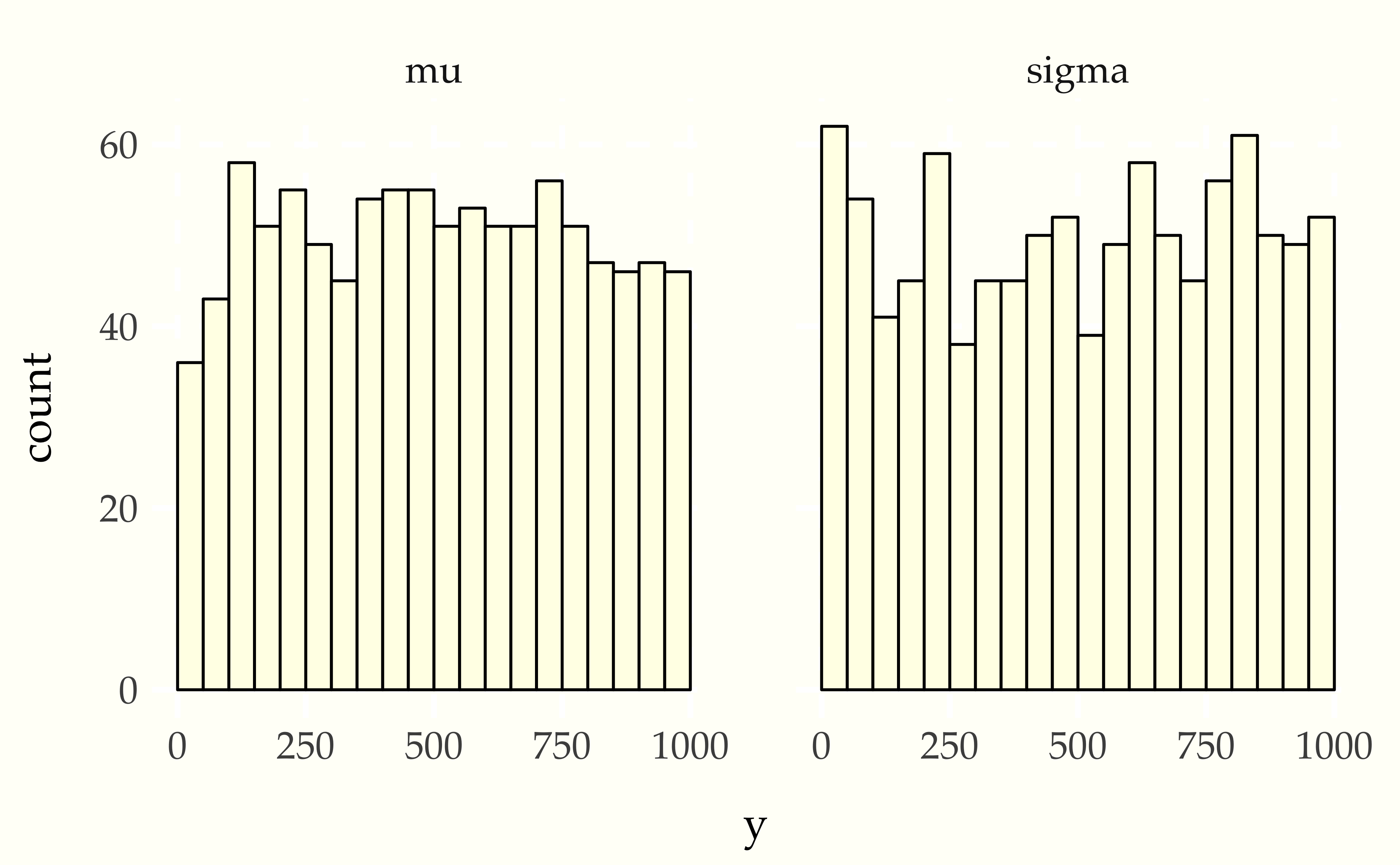
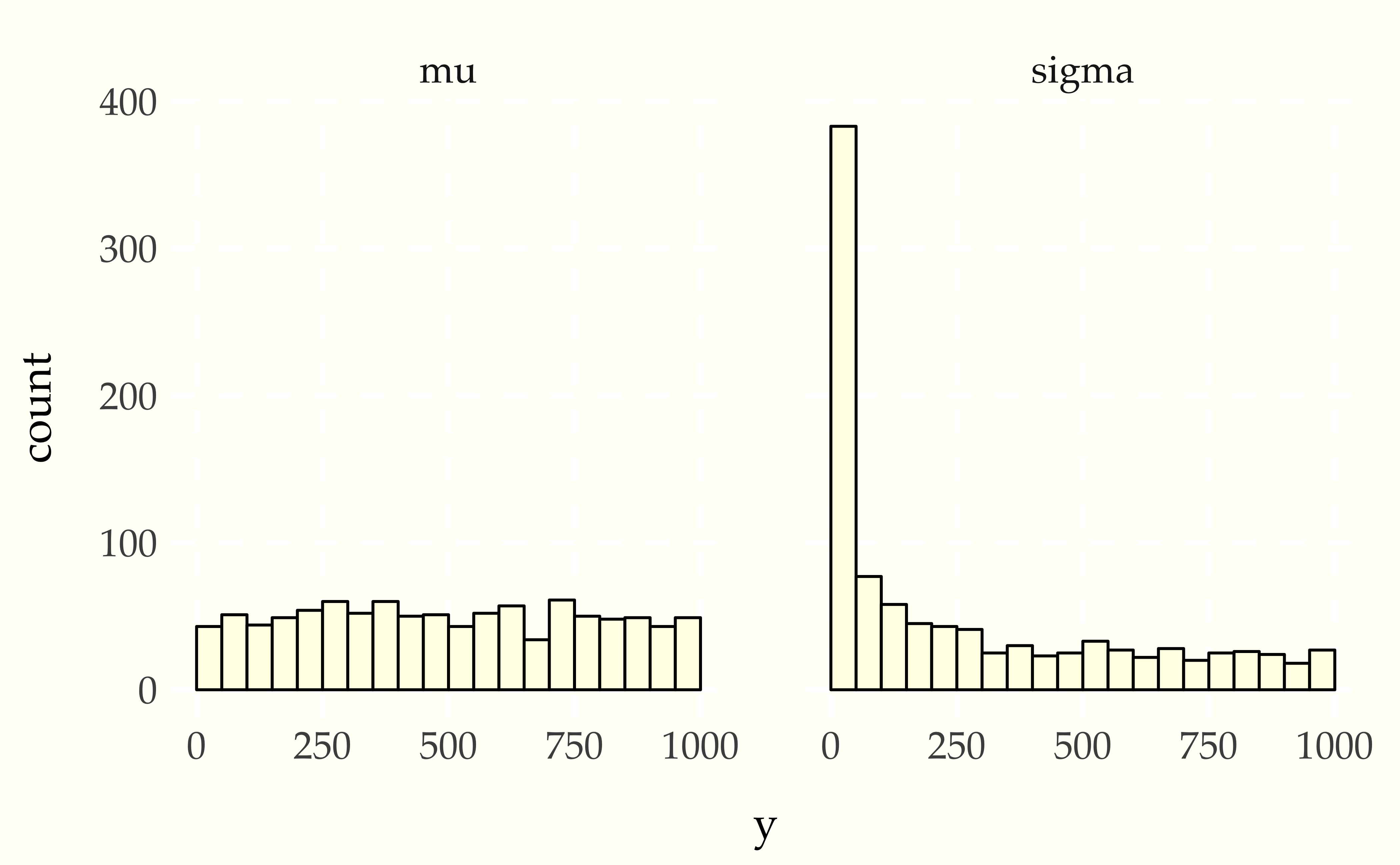
When things go wrong
当出现问题时
Now consider using a Student-t data generating process with a normal model. Compare the apparent uniformity of the well specified model with the ill-specified situation with Student-t generative process and normal model.
现在考虑使用 Student-t 数据生成过程配合正态模型。比较良好设定模型的表观均匀性与 Student-t 生成过程和正态模型的错误设定情况。
When Stan’s sampler goes wrong
当 Stan 的采样器出错时
The example in the previous sections show hard-coded pathological behavior. The usual application of SBC is to diagnose problems with a sampler.
前面章节中的示例显示了硬编码的病理行为。SBC 的通常应用是诊断采样器的问题。
This can happen in Stan with well-specified models if the posterior geometry is too difficult (usually due to extreme stiffness that varies). A simple example is the eight schools problem, the data for which consists of sample means \(y_j\) and standard deviations \(\sigma_j\) of differences in test score after the same intervention in \(J = 8\) different schools. Rubin (1981) applies a hierarchical model for a meta-analysis of the results, estimating the mean intervention effect and a varying effect for each school. With a standard parameterization and weak priors, this model has very challenging posterior geometry, as shown by Talts et al. (2018); this section replicates their results.
如果后验几何形状太困难(通常是由于极端的刚度变化),这可能会在 Stan 中发生在良好指定的模型上。一个简单的例子是八所学校问题,其数据包括 \(J = 8\) 所不同学校相同干预后测试分数差异的样本均值 \(y_j\) 和标准差 \(\sigma_j\)。Rubin (1981) 应用分层模型对结果进行元分析,估计平均干预效果和每所学校的变化效果。具有标准参数化和弱先验,该模型具有非常具有挑战性的后验几何形状,如 Talts et al. (2018) 所示;本节复制了他们的结果。
The meta-analysis model has parameters for a population mean \(\mu\) and standard deviation \(\tau > 0\) as well as the effect \(\theta_j\) of the treatment in each school. The model has weak normal and half-normal priors for the population-level parameters,
元分析模型具有总体均值 \(\mu\) 和标准差 \(\tau > 0\) 的参数,以及每所学校治疗效果 \(\theta_j\)。该模型对总体水平参数具有弱正态和半正态先验,
\[\begin{eqnarray*} \mu & \sim & \textrm{normal}(0, 5) \\[4pt] \tau & \sim & \textrm{normal}_{+}(0, 5). \end{eqnarray*}\] School level effects are modeled as normal given the population parameters,
学校水平效应在给定总体参数的情况下建模为正态,
\[ \theta_j \sim \textrm{normal}(\mu, \tau). \] The data is modeled as in a meta-analysis, given the school effect and sample standard deviation in the school,
数据按元分析建模,给定学校效应和学校中的样本标准差,
\[ y_j \sim \textrm{normal}(\theta_j, \sigma_j). \]
This model can be coded in Stan with a data-generating process that simulates the parameters and then simulates data according to the parameters.
该模型可以在 Stan 中编码,使用数据生成过程模拟参数,然后根据参数模拟数据。
transformed data {
  real mu_sim = normal_rng(0, 5);
  real tau_sim = abs(normal_rng(0, 5));
  int<lower=0> J = 8;
  array[J] real theta_sim = normal_rng(rep_vector(mu_sim, J), tau_sim);
  array[J] real<lower=0> sigma = abs(normal_rng(rep_vector(0, J), 5));
  array[J] real y = normal_rng(theta_sim, sigma);
}
parameters {
  real mu;
  real<lower=0> tau;
  array[J] real theta;
}
model {
  tau ~ normal(0, 5);
  mu ~ normal(0, 5);
  theta ~ normal(mu, tau);
  y ~ normal(theta, sigma);
}
generated quantities {
  int<lower=0, upper=1> mu_lt_sim = mu < mu_sim;
  int<lower=0, upper=1> tau_lt_sim = tau < tau_sim;
  int<lower=0, upper=1> theta1_lt_sim = theta[1] < theta_sim[1];
}
As usual for simulation-based calibration, the transformed data encodes the data-generating process using random number generators. Here, the population parameters \(\mu\) and \(\tau\) are first simulated, then the school-level effects \(\theta\), and then finally the observed data \(\sigma_j\) and \(y_j.\) The parameters and model are a direct encoding of the mathematical presentation using vectorized sampling statements. The generated quantities block includes indicators for parameter comparisons, saving only \(\theta_1\) because the schools are exchangeable in the simulation.
像往常一样,对于基于模拟的校准,transformed data 使用随机数生成器编码数据生成过程。这里,首先模拟总体参数 \(\mu\) 和 \(\tau\),然后是学校水平效应 \(\theta\),最后是观测数据 \(\sigma_j\) 和 \(y_j\)。参数和模型是使用向量化采样语句对数学表示的直接编码。generated quantities 块包括参数比较的指示器,仅保存 \(\theta_1\),因为学校在模拟中是可交换的。
When fitting the model in Stan, multiple warning messages are provided that the sampler has diverged. The divergence warnings are in Stan’s sampler precisely to diagnose the sampler’s inability to follow the curvature in the posterior and provide independent confirmation that Stan’s sampler cannot fit this model as specified.
在 Stan 中拟合模型时,会提供多个警告消息,表明采样器已发散。Stan 采样器中的发散警告正是为了诊断采样器无法跟随后验中的曲率,并提供独立确认,Stan 的采样器无法按指定拟合此模型。
SBC also diagnoses the problem. Here’s the rank plots for running \(N = 200\) simulations with 1000 warmup iterations and \(M = 999\) draws per simulation used to compute the ranks.
SBC 也诊断出了问题。这是运行 \(N = 200\) 次模拟的秩图,其中有 1000 次预热迭代和每次模拟用于计算秩的 \(M = 999\) 个抽样。
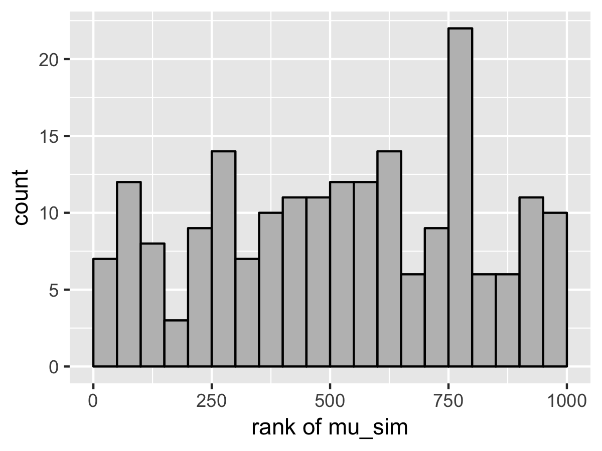
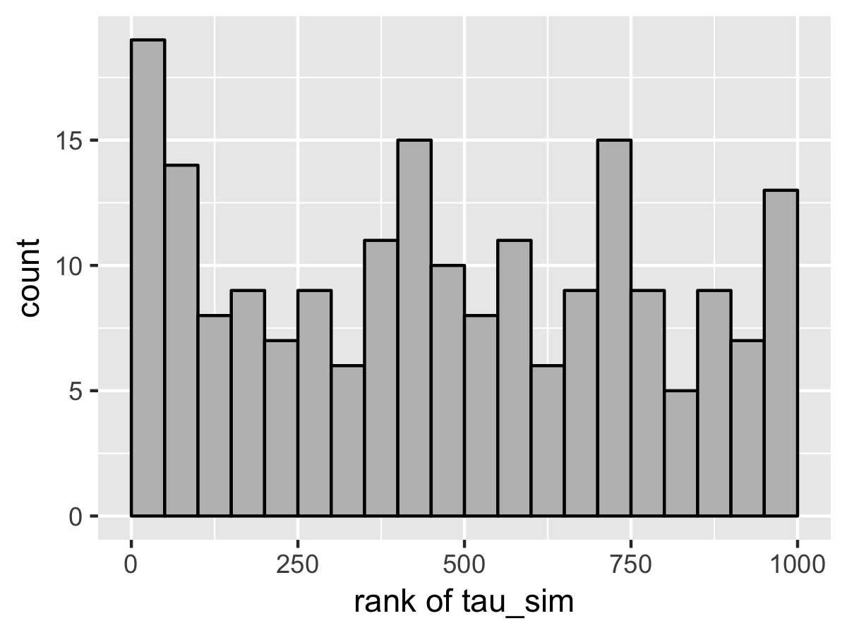
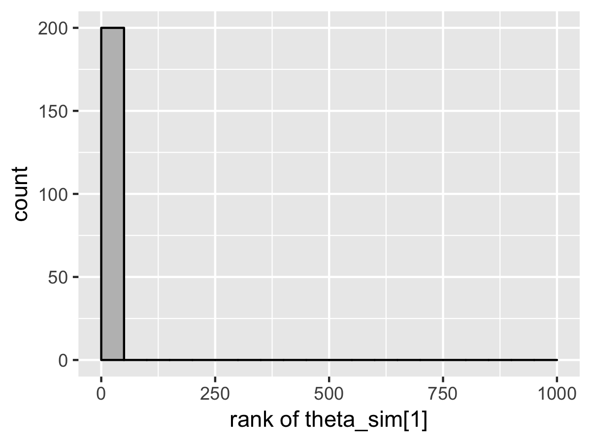
Although the population mean and standard deviation \(\mu\) and \(\tau\) appear well calibrated, \(\theta_1\) tells a very different story. The simulated values are much smaller than the values fit from the data. This is because Stan’s no-U-turn sampler is unable to sample with the model formulated in the centered parameterization—the posterior geometry has regions of extremely high curvature as \(\tau\) approaches zero and the \(\theta_j\) become highly constrained. The chapter on reparameterization explains how to remedy this problem and fit this kind of hierarchical model with Stan.
尽管总体均值和标准差 \(\mu\) 和 \(\tau\) 看起来校准良好,但 \(\theta_1\) 讲述了一个完全不同的故事。模拟值远小于从数据拟合的值。这是因为 Stan 的 no-U-turn 采样器无法使用中心参数化制定的模型进行采样——当 \(\tau\) 接近零且 \(\theta_j\) 变得高度受限时,后验几何形状具有极高曲率的区域。重参数化章节解释了如何解决这个问题并使用 Stan 拟合这种分层模型。