14 常微分方程
Ordinary Differential Equations
本节译者:杨静远
本节校审:张梓源(ChatGPT辅助)
Stan provides a number of different methods for solving systems of ordinary differential equations (ODEs). All of these methods adaptively refine their solutions in order to satisfy given tolerances, but internally they handle calculations quite a bit differently.
Stan 提供了多种不同的方法来求解常微分方程组(ODEs)。这些方法都能自适应地细化其解,以满足给定的容差要求。但它们的内部计算处理方式有所不同。
Because Stan’s algorithms requires gradients of the log density, the ODE solvers must not only provide the solution to the ODE itself, but also the gradient of the ODE solution with respect to parameters (the sensitivities). Two fundamentally different approaches are available in Stan to solve this problem, each having very different computational cost depending on the number of ODE states \(N\) and the number of parameters \(M\) being used:
因为 Stan 中的算法需要对对数密度的梯度进行求解,ODE 求解器不仅需要提供 ODE 本身的解,还要给出该解关于参数的梯度(即灵敏度)。在 Stan 中,针对该问题有两种本质上不同的方法可供选择,具体的计算成本取决于正在使用的 ODE 状态数量 \(N\) 和参数的数量 \(M\) 等因素:
A forward sensitivity solver expands the base ODE system with additional ODE equations for the gradients of the solution. For each parameter, an additional full set of \(N\) sensitivity states are added meaning that the full ODE solved has \(N \, + N \cdot M\) states.
前向灵敏度求解器通过为解的梯度添加额外的 ODE 方程,扩展了原始 ODE 系统。对于每个参数,都会添加一个完整的 \(N\) 个灵敏度状态,这意味着所解的完整 ODE 具有 \(N \, + N \cdot M\) 个状态。
An adjoint sensitivity solver starts by solving the base ODE system forward in time to get the ODE solution and then solves another ODE system (the adjoint) backward in time to get the gradients. The forward and reverse solves both have \(N\) states each. There is additionally one quadrature problem solved for every parameter.
伴随灵敏度求解器首先对基础 ODE 方程组进行正向求解,然后再对另一个 ODE 方程组(伴随方程)进行反向求解来获得梯度。正向和反向求解都各自拥有 \(N\) 个状态。此外,每个参数还需要单独求解一个求积问题。
The adjoint sensitivity approach scales much better than the forward sensitivity approach. Whereas the computational cost of the forward approach scales multiplicatively in the number of ODE states \(N\) and parameters \(M\), the adjoint sensitivity approach scales linear in states \(N\) and parameters \(M\). However, the adjoint problem is harder to configure and the overhead for small problems actually makes it slower than solving the full forward sensitivity system. With that in mind, the rest of this introduction focuses on the forward sensitivity interfaces. For information on the adjoint sensitivity interface see the Adjoint ODE solver
伴随灵敏度方法比正向灵敏度方法的可扩展性要好得多。虽然正向方法的计算成本随着 ODE 状态数 \(N\) 和参数数 \(M\) 成乘法关系增长,而伴随灵敏度方法的计算成本随着状态数 \(N\) 和参数数 \(M\) 线性增长。然而,伴随问题更难配置,对于小问题来说其开销使得伴随灵敏度算法比解决完整的正向灵敏度方程组更慢。考虑到这一点,本文余下的部分将重点介绍正向灵敏度接口。有关伴随灵敏度接口的信息,请参阅伴随 ODE 求解器。
Two interfaces are provided for each forward sensitivity solver: one with default tolerances and default max number of steps, and one that allows these controls to be modified. Choosing tolerances is important for making any of the solvers work well – the defaults will not work everywhere. The tolerances should be chosen primarily with consideration to the scales of the solutions, the accuracy needed for the solutions, and how the solutions are used in the model. For instance, if a solution component slowly varies between 3.0 and 5.0 and measurements of the ODE state are noisy, then perhaps the tolerances do not need to be as tight as for a situation where the solutions vary between 3.0 and 3.1 and very high precision measurements of the ODE state are available. It is also often useful to reduce the absolute tolerance when a component of the solution is expected to approach zero. For information on choosing tolerances, see the control parameters section.
每个正向灵敏度求解器都提供两个接口:一个带有默认容差和默认最大步数,一个允许用户自定义这些控制参数。选择容差对于使任何求解器正常工作都非常重要-默认值不适用于所有情况。容差的选择应主要考虑解的尺度、所需解的精度以及模型中使用解的方式。例如,如果解的分量在3.0和5.0之间缓慢变化,并且 ODE 状态的测量具有噪声,则容差可能不需要像解在3.0和3.1之间变化且可用高精度测量的情况下那么严格。当预计解的某个分量趋近于零时,减小绝对容差通常也很有用。有关选择容差的信息,请参阅控制参数部分。
The advantage of adaptive solvers is that as long as reasonable tolerances are provided and an ODE solver well-suited to the problem is chosen the technical details of solving the ODE can be abstracted away. The catch is that it is not always clear from the outset what reasonable tolerances are or which ODE solver is best suited to a problem. In addition, as changes are made to an ODE model, the optimal solver and tolerances may change.
自适应求解器的优点在于只要提供合理的容差并选择适合问题的 ODE 求解器,就可以将求解 ODE 的技术细节抽象出来。问题在于从一开始并不总是清楚什么是合理的容差或哪个 ODE 求解器最适合问题。此外,随着对 ODE 模型的更改,最佳求解器和容差可能会发生变化。
With this in mind, the four forward solvers are rk45, bdf, adams, and ckrk. If no other information about the ODE is available, start with the rk45 solver. The list below has information on when each solver is useful.
基于以上考虑,本文中介绍的四个正向求解器为 rk45、bdf、adams 和 ckrk。如果没有有关 ODE 的其他信息,请先选择 rk45 求解器。下面的列表提供了每个求解器适用情况的信息。
If there is any uncertainty about which solver is the best, it can be useful to measure the performance of all the interesting solvers using profile statements. It is difficult to always know exactly what solver is the best in all situations, but a profile can provide a quick check.
如果不确定哪个求解器是最适用的,那么使用 profile 语句对所有感兴趣的求解器来衡量其性能可能是有帮助的。在所有情况下都准确地了解哪个求解器是最优的是非常困难的,但是 profile 可以提供一个快速的检验。
rk45: a fourth and fifth order Runge-Kutta method for non-stiff systems (Dormand and Prince 1980; Ahnert and Mulansky 2011).rk45is the most generic solver and should be tried first.rk45:一种用于非刚性系统的四阶和五阶 Runge-Kutta 方法 (Dormand and Prince 1980; Ahnert and Mulansky 2011)。rk45是最通用的求解器,应该被优先尝试使用。bdf: a variable-step, variable-order, backward-differentiation formula implementation for stiff systems (Cohen and Hindmarsh 1996; Serban and Hindmarsh 2005).bdfis often useful for ODEs modeling chemical reactions.bdf:一种用于刚性系统的可变步长、可变阶数、后向差分公式实现 (Cohen and Hindmarsh 1996; Serban and Hindmarsh 2005)。bdf常用于模拟化学反应中的ODE。adams: a variable-step, variable-order, Adams-Moulton formula implementation for non-stiff systems (Cohen and Hindmarsh 1996; Serban and Hindmarsh 2005). The method has order up to 12, hence is commonly used when high-accuracy is desired for a very smooth solution, such as in modeling celestial mechanics and orbital dynamics (Montenbruck and Gill 2000).adams:一种用于非刚性系统的可变步长、可变阶数、Adams-Moulton 公式实现 (Cohen and Hindmarsh 1996; Serban and Hindmarsh 2005)。该方法的阶数高达12阶,因此在需要非常平滑的高精度解的情况下经常用于建模天体力学和轨道动力学 (Montenbruck and Gill 2000)。ckrk: a fourth and fifth order explicit Runge-Kutta method for non-stiff and semi-stiff systems (Cash and Karp 1990; Mazzia, Cash, and Soetaert 2012). The difference betweenckrkandrk45is thatckrkshould perform better for systems that exhibit rapidly varying solutions. Often in those situations the derivatives become large or even nearly discontinuous, andckrkis designed to address such problems.ckrk:一种用于非刚性和半刚性系统的四阶和五阶显式 Runge-Kutta 方法(Cash and Karp 1990; Mazzia, Cash, and Soetaert 2012)。ckrk与rk45的区别在于,在展示迅速变化的解的系统中,ckrk应该比rk45表现更好。在这些情况下,导数会变得很大,甚至几乎是不连续的,ckrk旨在解决这些问题。
For a discussion of stiff ODE systems, see the stiff ODE section. For information on the adjoint sensitivity interface see the Adjoint ODE solver section. The function signatures for Stan’s ODE solvers can be found in the function reference manual section on ODE solvers.
有关刚性 ODE 系统的讨论,请参见刚性 ODE 部分。有关伴随灵敏度接口的信息,请参见伴随 ODE 求解器部分。Stan 的 ODE 求解器的函数签名可以在函数参考手册中的 ODE 求解器部分找到。
14.1 Notation
符号
An ODE is defined by a set of differential equations, \(y(t, \theta)' = f(t, y, \theta)\), and initial conditions, \(y(t_0, \theta) = y_0\). The function \(f(t, y, \theta)\) is called the system function. The \(\theta\) dependence is included in the notation for \(y(t, \theta)\) and \(f(t, y, \theta)\) as a reminder that the solution is a function of any parameters used in the computation.
一个 ODE 是由一组微分方程定义的,\(y(t, \theta)' = f(t, y, \theta)\),以及初始条件 \(y(t_0, \theta) = y_0\)。函数 \(f(t, y, \theta)\) 被称作系统函数。\(\theta\) 的依赖关系被包含在 \(y(t, \theta)\) 和 \(f(t, y, \theta)\) 中以表示解是计算中用到的任意参数的一个函数。
14.2 Example: simple harmonic oscillator
示例:简谐振子
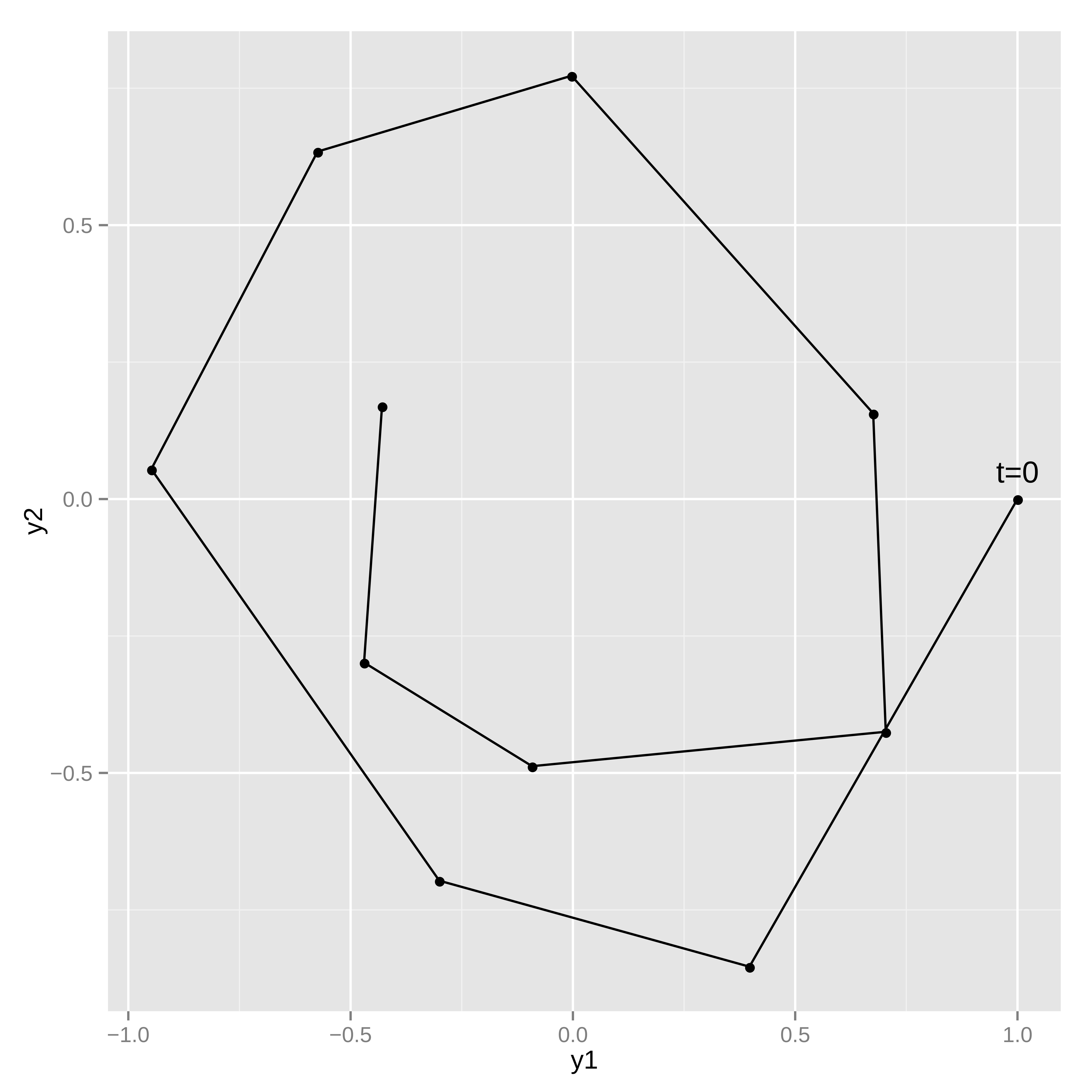
As an example of a system of ODEs, consider a harmonic oscillator. In a harmonic oscillator a particle disturbed from equilibrium is pulled back towards its equilibrium position by a force proportional to its displacement from equilibrium. The system here additionally has a friction force proportional to particle speed which points in the opposite direction of the particle velocity. The system state will be a pair \(y = (y_1, y_2)\) representing position and speed. The change in the system with respect to time is given by the following differential equations.1
作为一个 ODE 系统的示例,先考虑一个谐波振荡器。在谐波振荡器中,被扰乱平衡的粒子被一个与平衡位移成比例的力拉回其平衡位置。这里的系统还有一个与粒子速度成正比的摩擦力,它指向粒子速度的相反方向。系统的状态由表示位置和速度的 \(y = (y_1, y_2)\) 决定。系统相对于时间的变化由以下微分方程给出。2
\[\begin{align*} &\frac{d}{dt} y_1 = y_2 \\ &\frac{d}{dt} y_2 = -y_1 - \theta y_2 \end{align*}\]
The state equations implicitly defines the state at future times as a function of an initial state and the system parameters.
状态方程隐含地将未来时间的状态定义为一个初始状态和系统参数的函数。
14.3 Coding the ODE system function
ODE系统函数编程
The first step in coding an ODE system in Stan is defining the ODE system function. The system functions require a specific signature so that the solvers know how to use them properly.
在 Stan 中编写 ODE 系统的第一步是定义 ODE 系统函数。系统函数必须具有特定的函数签名,以便求解器能够正确调用它们。
The first argument to the system function is time, passed as a real; the second argument to the system function is the system state, passed as a vector, and the return value from the system function are the current time derivatives of the state defined as a vector. Additional arguments can be included in the system function to pass other information into the solve (these will be passed through the function that starts the ODE integration). These argument can be parameters (in this case, the friction coefficient), data, or any quantities that are needed to define the differential equation.
系统函数的第一个参数是时间,作为 real 传递;系统函数的第二个参数是系统状态,作为 vector 传递,并且系统函数的返回值是当前状态的时间导数,定义为 vector。可以在系统函数中包含其他参数以将其他信息传递给求解过程(这些参数将由启动 ODE 积分的函数传入)。这些参数可以是参数(在这种情况下是摩擦系数)、数据或任何需要定义微分方程的量。
The simple harmonic oscillator can be coded using the following function in Stan (see the user-defined functions chapter for more information on coding user-defined functions).
可以使用以下函数在 Stan 中编写简谐振子(有关编写用户定义函数的更多信息,请参见用户定义函数章节)。
vector sho(real t,        // time
           vector y,      // state
           real theta) {  // friction parameter
  vector[2] dydt;
  dydt[1] = y[2];
  dydt[2] = -y[1] - theta * y[2];
  return dydt;
}
The function takes in a time t (a real), the system state y (a vector), and the parameter theta (a real). The function returns a vector of time derivatives of the system state at time t, state y, and parameter theta. The simple harmonic oscillator coded here does not have time-sensitive equations; that is, t does not show up in the definition of dydt, however it is still required.
该函数接收时间 t(real)、系统状态 y(vector)和参数 theta(real)。该函数返回在时间 t、状态 y 和参数 theta 下的系统状态的时间导数的向量。此处编码的简谐振子不依赖时间变量;也就是说,t 未出现在 dydt 的定义中,但仍必须作为参数提供。
Strict signature
严格签名
The types in the ODE system function are strict. The first argument is the time passed as a real, the second argument is the state passed as a vector, and the return type is a vector. A model that does not have this signature will fail to compile. The third argument onwards can be any type, granted all the argument types match the types of the respective arguments in the solver call.
ODE 系统函数中的类型是严格的。第一个参数是作为实数传递的时间,第二个参数是作为向量传递的状态,返回类型是向量。不符合该签名的模型将无法通过编译。从第三个参数开始,可以是任何类型,只要所有参数类型与求解器调用中相应参数的类型匹配即可。
All of these are possible ODE signatures:
以下是可用的 ODE 签名:
vector myode1(real t, vector y, real a0);
vector myode2(real t, vector y, array[] int a0, vector a1);
vector myode3(real t, vector y, matrix a0, array[] real a1, row_vector a2);
but these are not allowed:
以下是不可用的签名:
vector myode1(real t, array[] real y, real a0);
// Second argument is not a vector
array[] real myode2(real t, vector y, real a0);
// Return type is not a vector
vector myode3(vector y, real a0);
// First argument is not a real and second is not a vector
14.4 Measurement error models
测量误差模型
Noisy observations of the ODE state can be used to estimate the parameters and/or the initial state of the system.
对 ODE 状态的噪声观测可以用来估计参数和/或系统的初始状态。
Simulating noisy measurements
噪声测量模拟
As an example, suppose the simple harmonic oscillator has a parameter value of \(\theta = 0.15\) and an initial state \(y(t = 0, \theta = 0.15) = (1, 0)\). Assume the system is measured at 10 time points, \(t = 1, 2, \cdots, 10\), where each measurement of \(y(t, \theta)\) has independent \(\textsf{normal}(0, 0.1)\) error in both dimensions (\(y_1(t, \theta)\) and \(y_2(t, \theta)\)).
作为示例,假设有一个带有参数值 \(\theta = 0.15\) 以及初始状态 \(y(t = 0, \theta = 0.15) = (1, 0)\) 的简谐振子。假设该系统在10个时间点进行了测量,\(t = 1, 2, \cdots, 10\),其中每个 \(y(t, \theta)\) 的观测值在两个分量上 (\(y_1(t, \theta)\) 和 \(y_2(t, \theta)\)) 都具有独立的 \(\textsf{normal}(0, 0.1)\) 噪声。
The following model can be used to generate data like this:
可以用下面的模型产生上述数据:
functions {
  vector sho(real t,
             vector y,
             real theta) {
    vector[2] dydt;
    dydt[1] = y[2];
    dydt[2] = -y[1] - theta * y[2];
    return dydt;
  }
}
data {
  int<lower=1> T;
  vector[2] y0;
  real t0;
  array[T] real ts;
  real theta;
}
model {
}
generated quantities {
  array[T] vector[2] y_sim = ode_rk45(sho, y0, t0, ts, theta);
  // add measurement error
  for (t in 1:T) {
    y_sim[t, 1] += normal_rng(0, 0.1);
    y_sim[t, 2] += normal_rng(0, 0.1);
  }
}
The system parameters theta and initial state y0 are read in as data along with the initial time t0 and observation times ts. The ODE is solved for the specified times, and then random measurement errors are added to produce simulated observations y_sim. Because the system is not stiff, the ode_rk45 solver is used.
系统参数 theta 和初始状态 y0 与初始时间 t0 和观测时间 ts 一起作为数据读入。ODE 在指定的时间内求解,然后添加随机测量误差以产生模拟观测值 y_sim。由于系统是非刚性的,因此选择 ode_rk45 求解器。
This program illustrates the way in which the ODE solver is called in a Stan program,
此程序说明了在 Stan 程序中调用 ODE 求解器的方式,
array[T] vector[2] y_sim = ode_rk45(sho, y0, t0, ts, theta);this returns the solution of the ODE initial value problem defined by system function sho, initial state y0, initial time t0, and parameter theta at the times ts. The call explicitly specifies the non-stiff RK45 solver.
此处的调用返回 ODE 初值问题的解,该问题由系统函数 sho、初始状态 y0、初始时间 t0 和参数 theta 在时间 ts 下定义。该调用明确指定使用非刚性 RK45 求解器
The parameter theta is passed unmodified to the ODE system function. If there were additional arguments that must be passed, they could be appended to the end of the ode call here. For instance, if the system function took two parameters, \(\theta\) and \(\beta\), the system function definition would look like:
参数 theta 未经修改地传递给 ODE 系统函数。如果有必须传递的其他参数,则可以将它们附加到此 ode 调用的末尾。例如,如果系统函数需要两个参数 \(\theta\) 和 \(\beta\),则系统函数定义将如下所示:
vector sho(real t, vector y, real theta, real beta) { ... }and the appropriate ODE solver call would be:
而适当的 ODE 求解器调用将为:
ode_rk45(sho, y0, t0, ts, theta, beta);Any number of additional arguments can be added. They can be any Stan type (as long as the types match between the ODE system function and the solver call).
可以添加任意数量的附加参数。它们可以是任何 Stan 类型(只要 ODE 系统函数和求解器调用之间的类型匹配)。
Because all none of the input arguments are a function of parameters, the ODE solver is called in the generated quantities block. The random measurement noise is added to each of the T outputs with normal_rng.
由于所有输入参数均为已知数据(即它们不依赖于模型参数),因此在 generated quantities 块中调用 ODE 求解器。使用 normal_rng 将随机测量噪声添加到每个 T 输出中。
Estimating system parameters and initial state
估计系统参数和初始状态
These ten noisy observations of the state can be used to estimate the friction parameter, \(\theta\), the initial conditions, \(y(t_0, \theta)\), and the scale of the noise in the problem. The full Stan model is:
这些带有噪声的十个状态观测可以用于估计摩擦参数 \(\theta\)、初始条件 \(y(t_0, \theta)\) 和问题中噪声的尺度。完整的 Stan 模型如下:
functions {
  vector sho(real t,
             vector y,
             real theta) {
    vector[2] dydt;
    dydt[1] = y[2];
    dydt[2] = -y[1] - theta * y[2];
    return dydt;
  }
}
data {
  int<lower=1> T;
  array[T] vector[2] y;
  real t0;
  array[T] real ts;
}
parameters {
  vector[2] y0;
  vector<lower=0>[2] sigma;
  real theta;
}
model {
  array[T] vector[2] mu = ode_rk45(sho, y0, t0, ts, theta);
  sigma ~ normal(0, 2.5);
  theta ~ std_normal();
  y0 ~ std_normal();
  for (t in 1:T) {
    y[t] ~ normal(mu[t], sigma);
  }
}
Because the solves are now a function of model parameters, the ode_rk45 call is now made in the model block. There are half-normal priors on the measurement error scales sigma, and standard normal priors on theta and the initial state vector y0. The solutions to the ODE are assigned to mu, which is used as the location for the normal observation model.
由于解现在是模型参数的函数,因此 ode_rk45 调用现在在模型块中进行。测量误差尺度 sigma 具有半正态先验,并且参数 theta 和初始状态向量 y0 具有标准正态先验。ODE 的解分配给 mu,并作为正态观测模型的均值项。
As with other regression models, it’s easy to change the noise model to something with heavier tails (e.g., Student-t distributed), correlation in the state variables (e.g., with a multivariate normal distribution), or both heavy tails and correlation in the state variables (e.g., with a multivariate Student-t distribution).
与其他回归模型类似,我们可以很容易地将噪声模型替换为具有更重尾部的分布(例如,Student-t 分布),状态变量具有相关性的分布(例如,使用多元正态分布),或同时具有重尾特性和变量相关性的分布(例如多元 Student-t 分布)。
14.5 Stiff ODEs
刚性 ODEs
Stiffness is a numerical phenomena that causes some differential equation solvers difficulty, notably the Runge-Kutta RK45 solver used in the examples earlier. The phenomena is common in chemical reaction systems, which are often characterized by having multiple vastly different time-scales. The stiffness of a system can also vary between different parts of parameter space, and so a typically non-stiff system may exhibit stiffness occasionally. These sorts of difficulties can occur more frequently with loose priors or during warmup.
刚性是一种数值现象,会使某些微分方程求解器面临计算上的困难,尤其是先前示例中使用的 Runge-Kutta RK45 求解器。这种现象在化学反应系统中很常见,这些系统通常具有多个截然不同的时间尺度。系统的刚性也可能因参数空间的不同部分而有所不同,因此通常非刚性的系统可能偶尔会表现出刚性。这些问题在使用宽松先验或模型预热阶段可能更频繁地出现。
Stan provides a specialized solver for stiff ODEs (Cohen and Hindmarsh 1996; Serban and Hindmarsh 2005). An ODE system is specified exactly the same way with a function of exactly the same signature. The only difference is in the call to the solver the rk45 suffix is replaced with bdf, as in
Stan 针对刚性 ODE 提供了专用求解器 (Cohen and Hindmarsh 1996; Serban and Hindmarsh 2005)。ODE 系统的定义方式与前述完全一致,使用完全相同签名的函数。唯一的区别在于,在调用求解器时,rk45 后缀被替换为 bdf,例如:
ode_bdf(sho, y0, t0, ts, theta);Using the stiff (bdf) solver on a system that is not stiff may be much slower than using the non-stiff (rk45) solver because each step of the stiff solver takes more time to compute. On the other hand, attempting to use the non-stiff solver for a stiff system will cause the timestep to become very small, leading the non-stiff solver taking more time overall even if each step is easier to compute than for the stiff solver.
对于非刚性系统,使用刚性(bdf)求解器可能比使用非刚性(rk45)求解器慢得多,因为每个刚性求解器的步骤需要更长时间来计算。另一方面,尝试在刚性系统上使用非刚性求解器将导致时间步长变得非常小,即使对于非刚性求解器,每个步骤比刚性求解器易于计算,但总体上需要更长的时间。
If it is not known for sure that an ODE system is stiff, run the model with both the rk45 and bdf solvers and see which is faster. If the rk45 solver is faster, then the problem is probably non-stiff, and then it makes sense to try the adams solver as well. The adams solver uses higher order methods which can take larger timesteps than the rk45 solver, though similar to the bdf solver each of these steps is more expensive to compute.
如果不确定 ODE 系统是否具有刚性,请使用 rk45 和 bdf 求解器运行模型,并查看哪个更快。如果 rk45 求解器更快,那么这个问题可能是非刚性的,此时尝试使用 adams 求解器也是合理的选择。adams 求解器使用更高阶方法,可以比 rk45 求解器采用更大的时间步长,尽管与 bdf 求解器类似,adams 求解器的每一步也更耗费计算资源。
14.6 Control parameters for ODE solving
ODE 求解中的控制参数
For additional control of the solves, both the stiff and non-stiff forward ODE solvers have function signatures that makes it possible to specify the relative_tolerance, absolute_tolerance, and max_num_steps parameters. These are the same as the regular function names but with _tol appended to the end. All three control arguments must be supplied with this signature (there are no defaults).
为了进一步控制求解过程,Stan 提供的刚性与非刚性前向 ODE 求解器都支持带有特定函数签名的版本,使用户可以显式指定 relative_tolerance、absolute_tolerance 和 max_num_steps 等控制参数。这些函数与常规版本的函数名称相同,但在末尾加上 _tol 后缀。使用该函数签名时,三个控制参数都必须显式提供(不设默认值)。
array[T] vector[2] y_sim = ode_bdf_tol(sho, y0, t0, ts,
                                 relative_tolerance,
                                 absolute_tolerance,
                                 max_num_steps,
                                 theta);
relative_tolerance and absolute_tolerance control accuracy the solver tries to achieve, and max_num_steps specifies the maximum number of steps the solver will take between output time points before throwing an error.
relative_tolerance 和 absolute_tolerance 控制求解器尝试达到的精度,max_num_steps 则指定在两个输出时间点之间,求解器最多允许执行的步数,超过该步数将抛出错误。
The control parameters must be data variables – they cannot be parameters or expressions that depend on parameters, including local variables in any block other than transformed data and generated quantities. User-defined function arguments may be qualified as only allowing data arguments using the data qualifier.
这些控制参数必须是数据变量 – 它们不能是参数或依赖于参数的表达式,包括 transformed data 和 generated quantities 以外的任何块中的局部变量。用户定义的函数参数可以使用 data 限定符限定为仅允许数据参数。
For the RK45 and Cash-Karp solvers, the default values for relative and absolute tolerance are both \(10^{-6}\) and the maximum number of steps between outputs is one million. For the BDF and Adams solvers, the relative and absolute tolerances are \(10^{-10}\) and the maximum number of steps between outputs is one hundred million.
对于 RK45 和 Cash-Karp 求解器,默认的相对和绝对容差值都为 \(10^{-6}\),在输出之间的最大迭代步数为一百万。对于BDF 和 Adams 求解器,相对和绝对容差为 \(10^{-10}\),在输出之间的最大迭代步数为一亿。
Discontinuous ODE system function
不连续 ODE 系统函数
If there are discontinuities in the ODE system function, it is best to integrate the ODE between the discontinuities, stopping the solver at each one, and restarting it on the other side.
如果 ODE 系统函数中存在间断点,最佳做法是仅在间断点之间对 ODE 进行积分,在每个间断点处停止求解器,并在间断点之后重新启动积分。
Nonetheless, the ODE solvers will attempt to integrate over discontinuities they encounters in the state function. The accuracy of the solution near the discontinuity may be problematic (requiring many small steps). An example of such a discontinuity is a lag in a pharmacokinetic model, where a concentration is zero for times \(0 < t < t'\) and then positive for \(t \geq t'\). In this example example, we would use code in the system such as
尽管如此,ODE 求解器仍会尝试在状态函数中遇到的间断点上进行积分。在间断点附近,解的精度可能会存在问题(需要非常小的步长)。这种间断的一个例子是药代动力学模型中的滞后现象,即当 \(0 < t < t'\) 时浓度为零,而在 \(t \geq t'\) 时变为正值。在这种情况下,我们可以在系统函数中编写如下代码:
if (t < t_lag) {
  return [0, 0]';
} else {
  // ... return non-zero vector...
}
In general it is better to integrate up to t_lag in one solve and then integrate from t_lag onwards in another. Mathematically, the discontinuity can make the problem ill-defined and the numerical integrator may behave erratically around it.
通常最好通过一次求解来积分到 t_lag,然后在 t_lag 之后重新开始积分。从数学上讲,间断点可能导致问题在数学上变得不适定,数值积分器在其周围的行为可能会出现异常。
If the location of the discontinuity cannot be controlled precisely, or there is some other rapidly change in ODE behavior, it can be useful to tell the ODE solver to produce output in the neighborhood. This can help the ODE solver avoid indiscriminately stepping over an important feature of the solution.
如果无法精确控制间断点的位置,或者其他 ODE 行为会快速变化,可以告诉 ODE 求解器在附近产生输出以帮助其避免不加区分地跨越解的重要特征。
Tolerance
容差
The relative tolerance RTOL and absolute tolerance ATOL control the accuracy of the numerical solution. Specifically, when solving an ODE with unknowns \(y=(y_1,\dots,y_n)^T\), at every step the solver controls estimated local error \(e=(e_1,\dots,e_n)^T\) through its weighted root-mean-square norm (Serban and Hindmarsh (2005), Hairer, Nørsett, and Wanner (1993))by reducing the stepsize when the inequality is not satisfied.
相对容差 RTOL 和绝对容差 ATOL 控制数值解的精度。具体地,在求解具有未知量 \(y=(y_1,\dots,y_n)^T\) 的 ODE 时,每一步求解器通过减小步长来控制加权均方根范数估计(Serban and Hindmarsh (2005), Hairer, Nørsett, and Wanner (1993))的局部误差 \(e=(e_1,\dots,e_n)^T\),直到不满足不等式
\[\begin{equation*} \sqrt{\sum_{i=1}^n{\frac{1}{n}\frac{e_i^2}{(\text{RTOL}\times y_i + \text{ATOL})^2}}} < 1 \end{equation*}\]
To understand the roles of the two tolerances it helps to assume \(y\) at opposite scales in the above expression: on one hand the absolute tolerance has little effect when \(y_i \gg 1\), on the other the relative tolerance can not affect the norm when \(y_i = 0\). Users are strongly encouraged to carefully choose tolerance values according to the ODE and its application. One can follow Brenan, Campbell, and Petzold (1995) for a rule of thumb: let \(m\) be the number of significant digits required for \(y\), set \(\text{RTOL}=10^{-(m+1)}\), and set ATOL at which \(y\) becomes insignificant. Note that the same weighted root-mean-square norm is used to control nonlinear solver convergence in bdf and adams solvers, and the same tolerances are used to control forward sensitivity calculation. See Serban and Hindmarsh (2005) for details.
为了理解这两个容差的作用不妨假设上述表达式中的 \(y\) 处于相反的尺度: 从一方面讲,当 \(y_i \gg 1\) 时,绝对容差几乎不起作用;另一方面,当 \(y_i = 0\) 时,相对容差不会影响范数。强烈建议用户根据 ODE 及其应用仔细选择容差值。可以按照 Brenan, Campbell, and Petzold (1995) 的经验法则:假设 \(y\) 所需的有效数字位数为 \(m\),则设置 \(\text{RTOL}=10^{-(m+1)}\),并将 ATOL 设置为导致 \(y\) 变得无意义的值。请注意,相同的加权均方根范数用于控制 bdf 和 adams 求解器中非线性求解器的收敛性,并且使用相同的容差来控制前向灵敏度计算。有关详细信息,请参见 Serban and Hindmarsh (2005) 。
Maximum number of steps
最大步数
The maximum number of steps can be used to stop a runaway simulation. This can arise in when MCMC moves to a part of parameter space very far from where a differential equation would typically be solved. In particular this can happen during warmup. With the non-stiff solver, this may happen when the sampler moves to stiff regions of parameter space, which will requires small step sizes.
设置最大迭代步数可以防止模拟过程失控。这可能发生在 MCMC 移动到参数空间中离通常求解微分方程的区域非常远的情况下。特别是在预热期间可能会发生这种情况。对于非刚性求解器,当采样器移动到参数空间的刚性区域时(需要较小的步长),这种情况可能会发生。
14.7 Adjoint ODE solver
伴随 ODE 求解器
The adjoint ODE solver method differs mathematically from the forward ODE solvers in the way gradients of the ODE solution are obtained. The forward ODE approach augments the original ODE system with \(N\) additional states for each parameter for which gradients are needed. If there are \(M\) parameters for which sensitivities are required, then the augmented ODE system has a total of \(N \cdot (M + 1)\) states. This can result in very large ODE systems through the multiplicative scaling of the computational effort needed.
在数学上,伴随 ODE 求解方法与正向求解方法在计算 ODE 解的梯度方式上存在本质差异。正向 ODE 方法对需要梯度的每个参数增加了 \(N\) 个附加状态。如果需要 \(M\) 个参数的灵敏度,则增加的 ODE 系统总共具有 \(N \cdot (M + 1)\) 个状态。这可能会导致 ODE 系统变得非常大,因为所需的计算工作量会成倍地增加。
In contrast, the adjoint ODE solver integrates forward in time a system of \(N\) equations to compute the ODE solution and then integrates backwards in time another system of \(N\) equations to get the sensitivities. Additionally, for \(M\) parameters there are \(M\) additional equations to integrate during the backwards solve. Because of this the adjoint sensitivity problem scales better in parameters than the forward sensitivity problem. The adjoint solver in Stan uses CVODES (the same as the bdf and adams forward sensitivity interfaces).
相比之下,伴随 ODE 求解器在时间上前向积分了一个包含 \(N\) 个方程的系统来计算 ODE 解,并在时间上后向积分另一个包含 \(N\) 个方程的系统来获取灵敏度。此外,对于需要 \(M\) 个参数的情况,在后向求解期间还有 \(M\) 个额外的方程需要积分。因此,伴随灵敏度方法在参数数量增加时具有更好的可扩展性。Stan 中的伴随求解器使用 CVODES(与 bdf 和 adams 正向灵敏度接口相同)。
The solution computed in the forward integration is required during the backward integration. CVODES uses a checkpointing scheme that saves the forward solver state regularly. The number of steps between saving checkpoints is configurable in the interface. These checkpoints are then interpolated during the backward solve using one of two interpolation schemes.
在前向积分中计算的解必须在后向积分中使用。CVODES 使用采用检查点机制定期保存前向求解器的状态。在接口中,可以配置保存检查点之间的步数。然后,后向求解期间,这些检查点将通过两种插值方法之一进行插值还原。
The solver type (either bdf or adams) can be individually set for both the forward and backward solves.
求解器类型(bdf 或 adams)可以分别设置为前向求解和后向求解。
The tolerances for each phase of the solve must be specified in the interface. Note that the absolute tolerance for the forward and backward ODE integration phase need to be set for each ODE state separately. The harmonic oscillator example call from above becomes:
必须在接口中指定每个求解阶段的容差。请注意,需要为每个 ODE 状态单独设置前向和后向 ODE 积分阶段的绝对容差。上面的谐波振荡器示例调用如下:
array[T] vector[2] y_sim
    = ode_adjoint_tol_ctl(sho, y0, t0, ts,
                          relative_tolerance/9.0,                // forward tolerance
                          rep_vector(absolute_tolerance/9.0, 2), // forward tolerance
                          relative_tolerance/3.0,                // backward tolerance
                          rep_vector(absolute_tolerance/3.0, 2), // backward tolerance
                          relative_tolerance,                    // quadrature tolerance
                          absolute_tolerance,                    // quadrature tolerance
                          max_num_steps,
                          150,                                   // number of steps between checkpoints
                          1,                                     // interpolation polynomial: 1=Hermite, 2=polynomial
                          2,                                     // solver for forward phase: 1=Adams, 2=BDF
                          2,                                     // solver for backward phase: 1=Adams, 2=BDF
                          theta);
For a detailed information on each argument please see the Stan function reference manual.
关于每个参数的详细信息,请参见 Stan 函数参考手册。
14.8 Solving a system of linear ODEs using a matrix exponential
用矩阵指数求解线性 ODE 系统
Linear systems of ODEs can be solved using a matrix exponential. This can be considerably faster than using one of the ODE solvers.
线性 ODE 系统可以通过矩阵指数形式求解。相较于数值积分法,这种方法在效率上更具优势。
The solution to \(\frac{d}{dt} y = ay\) is \(y = y_0e^{at}\), where the constant \(y_0\) is determined by boundary conditions. We can extend this solution to the vector case:
\(\frac{d}{dt} y = ay\) 的解为 \(y = y_0e^{at}\),其中 \(y_0\) 由边界条件决定。我们可以将此解扩展到向量情况:
\[ \frac{d}{dt}y = A \, y \] where \(y\) is now a vector of length \(n\) and \(A\) is an \(n\) by \(n\) matrix. The solution is then given by:
其中 \(y\) 是一个长度为\(n\)的向量,\(A\) 是一个 \(n \times n\) 的矩阵。此时,其通解为:
\[ y = e^{tA} \, y_0 \] where the matrix exponential is formally defined by the convergent power series:
其中矩阵指数是由收敛幂级数正式定义的:
\[ e^{tA} = \sum_{n=0}^{\infty} \dfrac{tA^n}{n!} = I + tA + \frac{t^2A^2}{2!} + \dotsb \]
We can apply this technique to the simple harmonic oscillator example, by setting
我们可以将这种技术应用于简单的谐波振荡器的例子,通过设置
\[ y = \begin{bmatrix} y_1 \\ y_2 \end{bmatrix} \qquad A = \begin{bmatrix} 0 & 1 \\ -1 & -\theta \end{bmatrix} \]
The Stan model to simulate noisy observations using a matrix exponential function is given below.
用矩阵指数函数模拟带有噪声观测的 Stan 模型如下所示。
In general, computing a matrix exponential will be more efficient than using a numerical solver. We can however only apply this technique to systems of linear ODEs.
通常情况下,计算矩阵指数将比使用数值求解器更有效。但是,我们只能将此技术应用于线性 ODE 系统。
data {
  int<lower=1> T;
  vector[2] y0;
  array[T] real ts;
  array[1] real theta;
}
model {
}
generated quantities {
  array[T] vector[2] y_sim;
  matrix[2, 2] A = [[ 0,  1],
                    [-1, -theta[1]]]
  for (t in 1:T) {
    y_sim[t] = matrix_exp((t - 1) * A) * y0;
  }
  // add measurement error
  for (t in 1:T) {
    y_sim[t, 1] += normal_rng(0, 0.1);
    y_sim[t, 2] += normal_rng(0, 0.1);
  }
}
This Stan program simulates noisy measurements from a simple harmonic oscillator. The system of linear differential equations is coded as a matrix. The system parameters theta and initial state y0 are read in as data along observation times ts. The generated quantities block is used to solve the ODE for the specified times and then add random measurement error, producing observations y_sim. Because the ODEs are linear, we can use the matrix_exp function to solve the system.
这个 Stan 程序模拟了一个简谐振子的带噪声的测量。线性微分方程组编码为矩阵形式。系统参数 theta 和初始状态 y0 作为数据与观测时间 ts 一起读入。generated quantities 块用于在指定的时间内解决 ODE,然后添加随机测量误差,生成观测值 y_sim。由于 ODE 是线性的,我们可以使用 matrix_exp 函数来求解 ODE 系统。
This example is drawn from the documentation for the Boost Numeric Odeint library (Ahnert and Mulansky 2011), which Stan uses to implement the
rk45andckrksolver.↩︎本示例来自 Boost Numeric Odeint 库的文档 (Ahnert and Mulansky 2011),Stan 使用该库实现了
rk45和ckrk求解器。↩︎