31 后验和先验预测检查
Posterior and Prior Predictive Checks
本节译者:陈苑莹
初次校审:张梓源
二次校审:邱怡轩(Claude Code+GLM 辅助)
Posterior predictive checks are a way of measuring whether a model does a good job of capturing relevant aspects of the data, such as means, standard deviations, and quantiles (Rubin 1984; Andrew Gelman, Meng, and Stern 1996). Posterior predictive checking works by simulating new replicated data sets based on the fitted model parameters and then comparing statistics applied to the replicated data set with the same statistic applied to the original data set.
后验预测检验是一种衡量模型是否能够很好地捕获数据相关特征的方法,如均值、标准差和分位数等 (Rubin 1984; Andrew Gelman, Meng, and Stern 1996)。基于拟合模型参数模拟产生新的复制数据集,然后将应用于复制数据集的统计量与应用于原始数据集的相同统计量进行比较。
Prior predictive checks evaluate the prior the same way. Specifically, they evaluate what data sets would be consistent with the prior. They will not be calibrated with actual data, but extreme values help diagnose priors that are either too strong, too weak, poorly shaped, or poorly located.
先验预测检查用同样的方式评估先验信息。具体来说,是评估哪些数据集与先验信息一致。 该方法不会使用实际数据进行校准,但极端值有助于诊断先验信息是否太强、太弱、形状不合适或位置不正确。
Prior and posterior predictive checks are two cases of the general concept of predictive checks, just conditioning on different things (no data and the observed data, respectively). For hierarchical models, there are intermediate versions, as discussed in the section on hierarchical models and mixed replication.
先验和后验预测检查是广义预测检查的两种情况,它们只是基于不同的条件(分别是无数据和观测数据)。对于分层模型,存在一些过渡形式的预测检查,具体讨论见分层模型和混合复制一节。
31.1 Simulating from the posterior predictive distribution
模拟后验预测分布
The posterior predictive distribution is the distribution over new observations given previous observations. It’s predictive in the sense that it’s predicting behavior on new data that is not part of the training set. It’s posterior in that everything is conditioned on observed data \(y\).
后验预测分布是基于先前观测到的数据来预测新观测数据的分布。从某种意义上说,它是预测性的,因为它预测了不属于训练集的新数据的特征;它也是后验的,因为一切都以观测到的数据 \(y\) 为条件。
The posterior predictive distribution for replications \(y^{\textrm{rep}}\) of the original data set \(y\) given model parameters \(\theta\) is defined by
原始数据集 \(y\) 的复制数据集 \(y^{\textrm{rep}}\) 在给定模型参数 \(\theta\) 下的后验预测分布定义为 \[ p(y^{\textrm{rep}} \mid y) = \int p(y^{\textrm{rep}} \mid \theta) \cdot p(\theta \mid y) \, \textrm{d}\theta. \]
As with other posterior predictive quantities, generating a replicated data set \(y^{\textrm{rep}}\) from the posterior predictive distribution is straightforward using the generated quantities block. Consider a simple regression model with parameters \(\theta = (\alpha, \beta, \sigma).\)
与其他后验预测量一样,使用 generated quantities 代码块可以直接从后验预测分布生成一个复制数据集 \(y^{\textrm{rep}}\)。考虑一个参数为 \(\theta = (\alpha, \beta, \sigma)\) 的简单回归模型。
data {
  int<lower=0> N;
  vector[N] x;
  vector[N] y;
}
parameters {
  real alpha;
  real beta;
  real<lower=0> sigma;
}
model {
  alpha ~ normal(0, 2);
  beta ~ normal(0, 1);
  sigma ~ normal(0, 1);
  y ~ normal(alpha + beta * x, sigma);
}
To generate a replicated data set y_rep for this simple model, the following generated quantities block suffices.
要为这个简单模型生成一个复制数据集 y_rep,使用下面这个 generated quantities 代码块即可。
generated quantities {
  array[N] real y_rep = normal_rng(alpha + beta * x, sigma);
}
The vectorized form of the normal random number generator is used with the original predictors x and the model parameters alpha, beta, and sigma. The replicated data variable y_rep is declared to be the same size as the original data y, but instead of a vector type, it is declared to be an array of reals to match the return type of the function normal_rng. Because the vector and real array types have the same dimensions and layout, they can be plotted against one another and otherwise compared during downstream processing.
使用正态随机数生成器的向量化形式,配合原始预测变量 x 和模型参数 alpha, beta, sigma 生成数据。复制数据变量 y_rep 与原始数据 y 维度相同,但为了匹配 normal_rng 函数的返回类型,它声明为实数数组而非向量类型。由于向量和实数数组具有相同的维度和布局,因此在后续处理中可以对它们进行绘图和比较。
The posterior predictive sampling for posterior predictive checks is different from usual posterior predictive sampling discussed in the chapter on posterior predictions in that the original predictors \(x\) are used. That is, the posterior predictions are for the original data.
后验预测检查的后验预测采样与后验预测一章中讨论的通常后验预测采样不同之处在于使用了原始预测变量 \(x\)。也就是说,后验预测是针对原始数据的。
31.2 Plotting multiples
多图绘制
A standard posterior predictive check would plot a histogram of each replicated data set along with the original data set and compare them by eye. For this purpose, only a few replications are needed. These should be taken by thinning a larger set of replications down to the size needed to ensure rough independence of the replications.
一个标准的后验预测检查会绘制每个复制数据集与原始数据集的直方图并进行直观比较。为此,只需要少量的复制数据集,可以通过抽稀一个较大的复制数据集集合来实现,只要能确保复制数据集之间大致独立即可。
Here’s a complete example where the model is a simple Poisson with a weakly informative exponential prior with a mean of 10 and standard deviation of 10.
下面是一个完整的示例,其中模型是一个简单的泊松分布,具有均值为10和标准差为10的弱信息指数先验分布。
data {
  int<lower=0> N;
  array[N] int<lower=0> y;
}
transformed data {
  real<lower=0> mean_y = mean(to_vector(y));
  real<lower=0> sd_y = sd(to_vector(y));
}
parameters {
  real<lower=0> lambda;
}
model {
  y ~ poisson(lambda);
  lambda ~ exponential(0.2);
}
generated quantities {
  array[N] int<lower=0> y_rep = poisson_rng(rep_array(lambda, N));
  real<lower=0> mean_y_rep = mean(to_vector(y_rep));
  real<lower=0> sd_y_rep = sd(to_vector(y_rep));
  int<lower=0, upper=1> mean_gte = (mean_y_rep >= mean_y);
  int<lower=0, upper=1> sd_gte = (sd_y_rep >= sd_y);
}
The generated quantities block creates a variable y_rep for the replicated data, variables mean_y_rep and sd_y_rep for the statistics of the replicated data, and indicator variables mean_gte and sd_gte for whether the replicated statistic is greater than or equal to the statistic applied to the original data.
generated quantities 代码块创建了复制数据变量 y_rep、复制数据的统计量变量 mean_y_rep 和 sd_y_rep,以及指示变量 mean_gte 和 sd_gte,用于表示复制数据的统计量是否大于或等于原始数据的统计量。
Now consider generating data \(y \sim \textrm{Poisson}(5)\). The resulting small multiples plot shows the original data plotted in the upper left and eight different posterior replications plotted in the remaining boxes.
现在考虑生成数据 \(y \sim \textrm{Poisson}(5)\)。生成的少量多图如下,原始数据集绘制在左上角,其余框中绘制了八个不同的后验复制数据集。

With a Poisson data-generating process and Poisson model, the posterior replications look similar to the original data. If it were easy to pick the original data out of the lineup, there would be a problem.
对于泊松数据生成过程和泊松模型,后验复制集看起来与原始数据集很相似。如果能够轻松地从多个数据集中区分出原始数据,那就会存在问题。
Now consider generating over-dispersed data \(y \sim \textrm{negative-binomial2}(5, 1).\) This has the same mean as \(\textrm{Poisson}(5)\), namely \(5\), but a standard deviation of \(\sqrt{5 + 5^2 /1} \approx 5.5.\) There is no way to fit this data with the Poisson model, because a variable distributed as \(\textrm{Poisson}(\lambda)\) has mean \(\lambda\) and standard deviation \(\sqrt{\lambda},\) which is \(\sqrt{5}\) for \(\textrm{Poisson}(5).\) Here’s the resulting small multiples plot, again with original data in the upper left.
现在考虑生成过度离散的数据 \(y \sim \textrm{negative-binomial2}(5, 1)\),其与 \(\textrm{Poisson}(5)\) 有相同的均值 \(5\),但是标准差不同,为 \(\sqrt{5 + 5^2 /1} \approx 5.5\)。此时无法用泊松模型去拟合这个数据,因为服从 \(\textrm{Poisson}(\lambda)\) 的变量均值为 \(\lambda\),标准差为 \(\sqrt{\lambda}\),这对于 \(\textrm{Poisson}(5)\) 来说就是 \(\sqrt{5}\)。下图是得到的少量多图,原始数据同样在左上角。
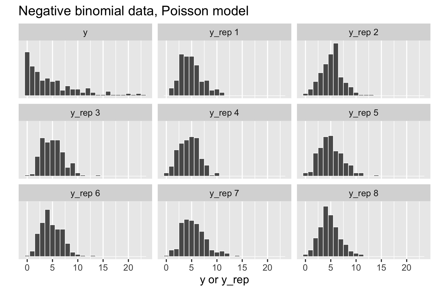
This time, the original data stands out in stark contrast to the replicated data sets, all of which are clearly more symmetric and lower variance than the original data. That is, the model’s not appropriately capturing the variance of the data.
这次,原始数据与所有复制数据集形成鲜明对比,所有复制数据集都明显比原始数据更对称且方差更小。也就是说,该模型未能很好地捕获到数据的方差。
31.3 Posterior ‘’p-values’’
后验 “p值”
If a model captures the data well, summary statistics such as sample mean and standard deviation, should have similar values in the original and replicated data sets. This can be tested by means of a p-value-like statistic, which here is just the probability the test statistic \(s(\cdot)\) in a replicated data set exceeds that in the original data,
如果一个模型很好地捕获了数据特征,那么原始数据和复制数据集中的一些汇总统计量(如样本均值和标准差)应该具有相似的值。这可以通过一个类似 p 值的统计量来检验,在这里它是复制数据集的检验统计量 \(s(\cdot)\) 超过原始数据集的概率, \[ \Pr\!\left[ s(y^{\textrm{rep}}) \geq s(y) \mid y \right] = \int \textrm{I}\left( s(y^{\textrm{rep}}) \geq s(y) \mid y \right) \cdot p\left( y^{\textrm{rep}} \mid y \right) \, \textrm{d}{y^{\textrm{rep}}}. \] It is important to note that ‘’p-values’’ is in quotes because these statistics are not classically calibrated, and thus will not in general have a uniform distribution even when the model is well specified (Bayarri and Berger 2000).
需要注意的是,“p值”是带引号的,因为这些统计量没有经过经典校准,因此即使模型设定正确,通常也不会具有均匀分布 (Bayarri and Berger 2000)。
Nevertheless, values of this statistic very close to zero or one are cause for concern that the model is not fitting the data well. Unlike a visual test, this p-value-like test is easily automated for bulk model fitting.
然而,当该统计量的值非常接近于0或1时,表明模型可能不能很好地拟合数据,需要引起关注。与视觉检验不同,这种类似 p 值的检验可以轻松地自动化处理,适用于批量模型拟合。
To calculate event probabilities in Stan, it suffices to define indicator variables that take on value 1 if the event occurs and 0 if it does not. The posterior mean is then the event probability. For efficiency, indicator variables are defined in the generated quantities block.
要在 Stan 中计算事件概率,只需定义指示变量即可:当事件发生时取值为1,否则取值为0。后验均值即为事件概率。为了提高效率,指示变量可以在 generated quantities 代码块中定义。
generated quantities {
  int<lower=0, upper=1> mean_gt;
  int<lower=0, upper=1> sd_gt;
  {
    array[N] real y_rep = normal_rng(alpha + beta * x, sigma);
    mean_gt = mean(y_rep) > mean(y);
    sd_gt = sd(y_rep) > sd(y);
  }
}
The indicator variable mean_gt will have value 1 if the mean of the simulated data y_rep is greater than or equal to the mean of he original data y. Because the values of y_rep are not needed for the posterior predictive checks, the program saves output space by using a local variable for y_rep. The statistics mean(u) and sd(y) could also be computed in the transformed data block and saved.
如果模拟数据 y_rep 的均值大于或等于原始数据 y 的均值,指示变量 mean_gt 取值为1。由于后验预测检查不需要 y_rep 的值,因此该程序通过对 y_rep 使用局部变量来节省输出空间。统计量 mean(y) 和 sd(y) 也可以在 transformed data 代码块中计算和保存。
For the example in the previous section, where over-dispersed data generated by a negative binomial distribution was fit with a simple Poisson model, the following plot illustrates the posterior p-value calculation for the mean statistic.
对于上一节中的例子,用一个简单的泊松模型拟合负二项分布产生的过度离散的数据,下图说明了均值统计量的后验 p 值计算。
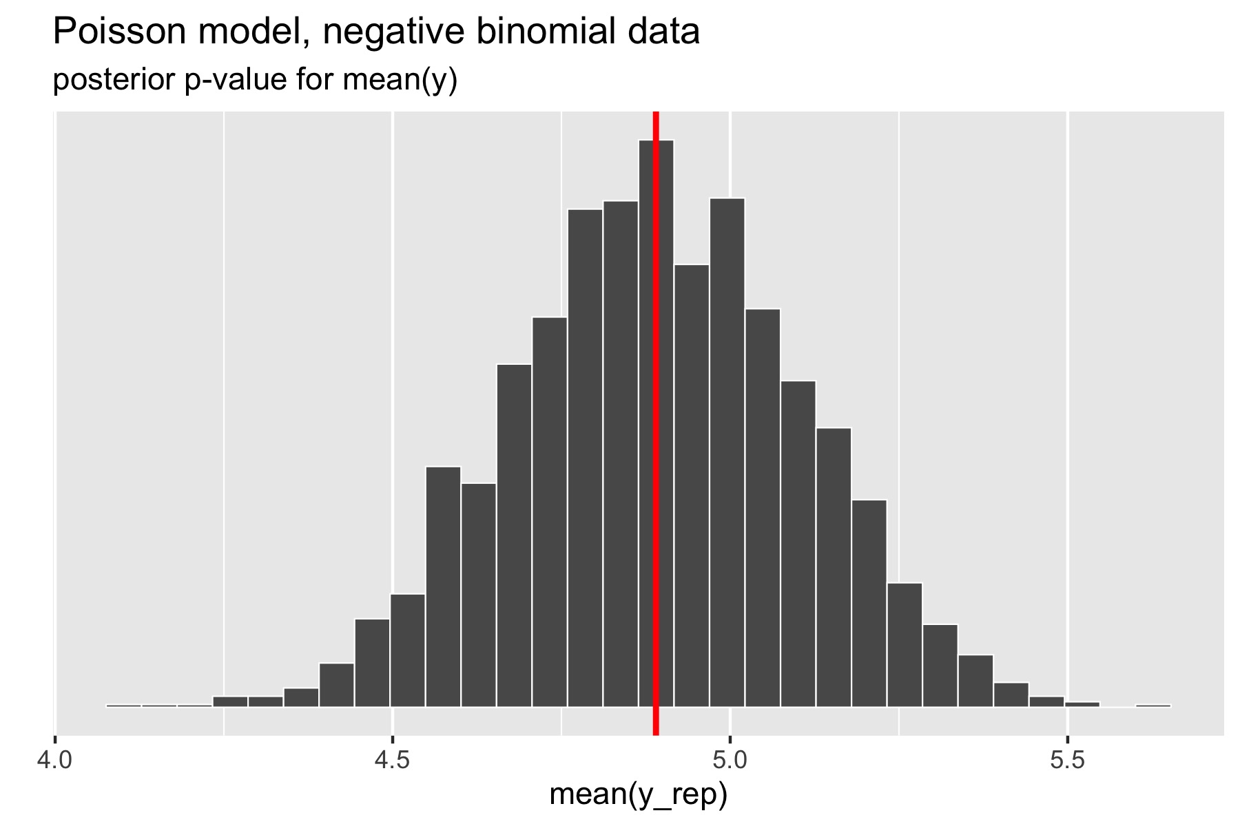
The p-value for the mean is just the percentage of replicated data sets whose statistic is greater than or equal that of the original data. Using a Poisson model for negative binomial data still fits the mean well, with a posterior \(p\)-value of 0.49. In Stan terms, it is extracted as the posterior mean of the indicator variable mean_gt.
均值的 p 值就是复制数据集的统计量大于或等于原始数据集的百分比。使用泊松模型仍然可以很好地拟合该负二项数据的均值,其后验 p 值为0.49。在 Stan 中,可以通过计算指示变量 mean_gt 的后验均值来得到该 p 值。
The standard deviation statistic tells a different story.
但标准差统计量呈现了一个截然不同的结果。
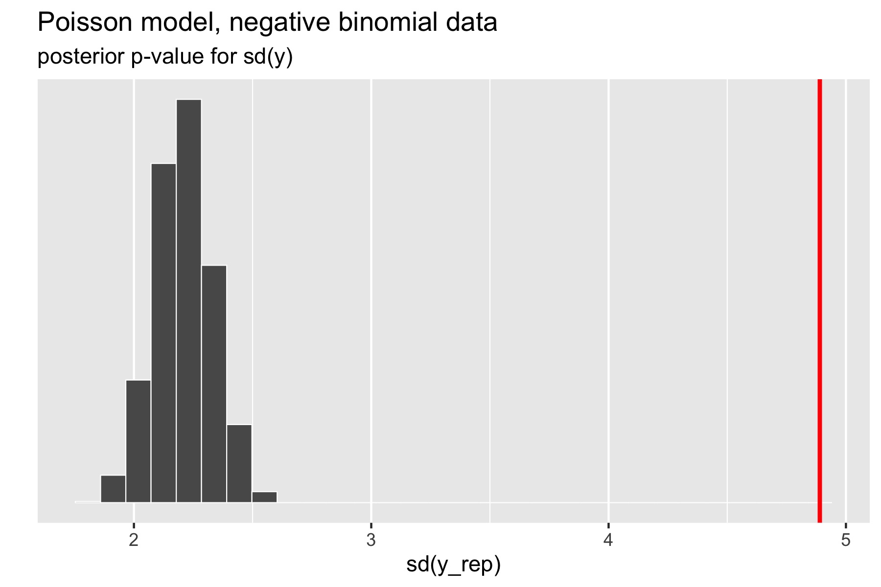
Here, the original data has much higher standard deviation than any of the replicated data sets. The resulting \(p\)-value estimated by Stan after a large number of iterations is exactly zero (the absolute error bounds are fine, but a lot of iterations are required to get good relative error bounds on small \(p\)-values by sampling). In other words, there were no posterior draws in which the replicated data set had a standard deviation greater than or equal to that of the original data set. Clearly, the model is not capturing the dispersion of the original data. The point of this exercise isn’t just to figure out that there’s a problem with a model, but to isolate where it is. Seeing that the data is over-dispersed compared to the Poisson model would be reason to fit a more general model like the negative binomial or a latent varying effects (aka random effects) model that can account for the over-dispersion.
这里,原始数据的标准差比任何复制数据集都要高得多。经过大量迭代后,Stan 估计产生的 \(p\) 值为零(绝对误差边界是可接受的,但需要大量迭代才能通过采样得到小 \(p\) 值的相对误差边界)。换句话说,没有后验采样点能使复制数据集的标准差大于或等于原始数据集的标准差。显然,该模型没有捕获到原始数据的离散性。这个练习的重点不仅仅是确定模型存在问题,而是要找出问题所在。观察到数据与泊松模型相比过于离散,就有理由采用更一般的模型,如负二项分布或潜在变化效应(又名随机效应)模型,这些模型能够解释过度离散的现象。
Which statistics to test?
检验哪个统计量?
Any statistic may be used for the data, but these can be guided by the quantities of interest in the model itself. Popular choices in addition to mean and standard deviation are quantiles, such as the median, 5% or 95% quantiles, or even the maximum or minimum value to test extremes.
任何统计量都可以使用,但也可以根据模型本身感兴趣的量来选择。除了均值和标准差之外,常见的选择是分位数,例如中位数、5% 或 95% 分位数,还有检验极端值的最大值或最小值。
Despite the range of choices, test statistics should ideally be ancillary, in the sense that they should be testing something other than the fit of a parameter. For example, a simple normal model of a data set will typically fit the mean and variance of the data quite well as long as the prior doesn’t dominate the posterior. In contrast, a Poisson model of the same data cannot capture both the mean and the variance of a data set if they are different, so they bear checking in the Poisson case. As we saw with the Poisson case, the posterior mean for the single rate parameter was located near the data mean, not the data variance. Other distributions such as the lognormal and gamma distribution, have means and variances that are functions of two or more parameters.
尽管有各种选择,但理想情况下,检验统计量应该是辅助的,即它们应该测试除参数拟合之外的其他内容。例如,对于一个简单的正态模型,只要先验不主导后验,通常可以很好地拟合数据的均值和方差。相比之下,如果数据集的均值和方差不同,那么泊松模型就无法同时捕获到数据的均值和方差,因此在泊松模型中需要进行检验。正如我们在泊松模型中看到的那样,单个速率参数的后验均值位于数据均值附近,而不在数据方差附近。其他分布,如对数正态分布和伽马分布,均值和方差是两个或多个参数的函数。
31.4 Prior predictive checks
先验预测检查
Prior predictive checks generate data according to the prior in order to asses whether a prior is appropriate (Gabry et al. 2019). A posterior predictive check generates replicated data according to the posterior predictive distribution. In contrast, the prior predictive check generates data according to the prior predictive distribution,
先验预测检查根据先验分布生成数据,以评估先验分布是否合适 (Gabry et al. 2019)。后验预测检查根据后验预测分布生成复制数据集。相比之下,先验预测检查根据先验预测分布生成数据,
\[ y^{\textrm{sim}} \sim p(y). \] The prior predictive distribution is just like the posterior predictive distribution with no observed data, so that a prior predictive check is nothing more than the limiting case of a posterior predictive check with no data.
先验预测分布就像是没有观测数据的后验预测分布,因此,先验预测检查只不过是没有数据的后验预测检查的极限情况。
This is easy to carry out mechanically by simulating parameters
这很容易通过模拟参数来程序化地实现
\[ \theta^{\textrm{sim}} \sim p(\theta) \] according to the priors, then simulating data
根据先验信息,再模拟数据
\[ y^{\textrm{sim}} \sim p(y \mid \theta^{\textrm{sim}}) \] according to the data model given the simulated parameters. The result is a simulation from the joint distribution,
根据给定了模拟参数的抽样分布。结果是从联合分布进行模拟,
\[ (y^{\textrm{sim}}, \theta^{\textrm{sim}}) \sim p(y, \theta) \] and thus
因此
\[ y^{\textrm{sim}} \sim p(y) \] is a simulation from the prior predictive distribution.
是一个来自先验预测分布的模拟。
Coding prior predictive checks in Stan
在 Stan 中进行先验预测检查的编程
A prior predictive check is coded just like a posterior predictive check. If a posterior predictive check has already been coded and it’s possible to set the data to be empty, then no additional coding is necessary. The disadvantage to coding prior predictive checks as posterior predictive checks with no data is that Markov chain Monte Carlo will be used to sample the parameters, which is less efficient than taking independent draws using random number generation.
先验预测检查的编程方式与后验预测检查相同。如果已编写了后验预测检查代码,并且可以将数据设置为空,则无需额外编程。将先验预测检查编写为无数据的后验预测检查的缺点是会使用马尔可夫链蒙特卡罗对参数进行采样,这比使用随机数生成独立采样点的效率低。
Prior predictive checks can be coded entirely within the generated quantities block using random number generation. The resulting draws will be independent. Predictors must be read in from the actual data set—they do not have a generative model from which to be simulated. For a Poisson regression, prior predictive sampling can be encoded as the following complete Stan program.
先验预测检查可以完全在使用随机数生成器的 generated quantities 代码块内编写,生成的采样点将是独立的。预测变量必须从实际数据集中读取——它们没有一个生成模型可以进行模拟。对于泊松回归,先验预测采样可以编写为以下完整的 Stan 程序。
data {
  int<lower=0> N;
  vector[N] x;
}
generated quantities {
  real alpha = normal_rng(0, 1);
  real beta = normal_rng(0, 1);
  array[N] real y_sim = poisson_log_rng(alpha + beta * x);
}
Running this program using Stan’s fixed-parameter sampler yields draws from the prior. These may be plotted to consider their appropriateness.
使用 Stan 的固定参数采样器运行这个程序会产生来自先验的采样点。可以将这些采样点绘制出来以考虑其适用性。
31.5 Example of prior predictive checks
一个关于先验预测检查的示例
Suppose we have a model for a football (aka soccer) league where there are \(J\) teams. Each team has a scoring rate \(\lambda_j\) and in each game will be assumed to score \(\textrm{poisson}(\lambda_j)\) points. Yes, this model completely ignores defense. Suppose the modeler does not want to “put their thumb on the scale” and would rather “let the data speak for themselves” and so uses a prior with very wide tails, because it seems uninformative, such as the widely deployed
假设我们有一个足球联赛的模型,其中有 \(J\) 支队伍。每支队伍都有一个得分率 \(\lambda_j\),在每场比赛中的得分被认为服从 \(\textrm{poisson}(\lambda_j)\)。是的,该模型完全忽略防守。假设建模者不想“人为干预模型结果”,而宁愿“让数据自己说话”,因此使用了看起来似乎无信息性的宽尾先验,例如广泛使用的
\[ \lambda_j \sim \textrm{gamma}(\epsilon_1, \epsilon_2). \] This is not just a manufactured example; The BUGS Book recommends setting \(\epsilon = (0.5, 0.00001)\), which corresponds to a Jeffreys prior for a Poisson rate parameter prior (Lunn et al. 2012, 85).
这不仅仅是一个人为的例子;The BUGS Book建议设置 \(\epsilon = (0.5, 0.00001)\),这相当于一个泊松速率参数的 Jeffreys 先验 (Lunn et al. 2012, 85)。
Suppose the league plays a round-robin tournament wherein every team plays every other team. The following Stan model generates random team abilities and the results of such a round-robin tournament, which may be used to perform prior predictive checks.
假设联盟进行循环赛,每支球队都会与其他每支球队进行比赛。下面的 Stan 模型随机生成球队的能力和这种循环赛的结果,可以用来执行先验预测检查。
data {
  int<lower=0> J;
  array[2] real<lower=0> epsilon;
}
generated quantities {
  array[J] real<lower=0> lambda;
  array[J, J] int y;
  for (j in 1:J) lambda[j] = gamma_rng(epsilon[1], epsilon[2]);
  for (i in 1:J) {
    for (j in 1:J) {
      y[i, j] = poisson_rng(lambda[i]) - poisson_rng(lambda[j]);
    }
  }
}
In this simulation, teams play each other twice and play themselves once. This could be made more realistic by controlling the combinatorics to only generate a single result for each pair of teams, of which there are \(\binom{J}{2} = \frac{J \cdot (J - 1)}{2}.\)
在这个模拟中,各支队伍对战对方两次,对战自己一次。可以通过控制组合运算,使其更加逼真,只为 \(\binom{J}{2} = \frac{J \cdot (J - 1)}{2}\) 场中的每场比赛生成一个结果。
Using the \(\textrm{gamma}(0.5, 0.00001)\) reference prior on team abilities, the following are the first 20 simulated point differences for the match between the first two teams, \(y^{(1:20)}_{1, 2}\).
使用 \(\textrm{gamma}(0.5, 0.00001)\) 作为队伍能力的先验分布,下面是前两个队伍比赛的前20个模拟分差,\(y^{(1:20)}_{1, 2}\)。
2597 -26000   5725  22496   1270   1072   4502  -2809   -302   4987
7513   7527  -3268 -12374   3828   -158 -29889   2986  -1392     66
That’s some pretty highly scoring football games being simulated; all but one has a score differential greater than 100! In other words, this \(\textrm{gamma}(0.5, 0.00001)\) prior is putting around 95% of its weight on score differentials above 100. Given that two teams combined rarely score 10 points, this prior is way out of line with prior knowledge about football matches; it is not only consistent with outcomes that have never occurred in the history of the sport, it puts most of the prior probability mass there.
这些是模拟的一些得分极高的足球比赛;除了一个以外,所有分差都大于100!换句话说,这个 \(\textrm{gamma}(0.5, 0.00001)\) 先验分布将约95%的权重放在100分以上的分差上。考虑到两支球队合起来很少能得10分,这个先验与足球比赛的先验知识严重不符;它不仅与体育运动历史上从未发生过的结果一致,而且把大部分先验概率质量都放在了那里。
The posterior predictive distribution can be strongly affected by the prior when there is not much observed data and substantial prior mass is concentrated around infeasible values (A. Gelman 2006).
当观测数据不多,先验分布大量集中在不可行值周围时,后验预测分布会受到先验的强烈影响 (A. Gelman 2006)。
Just as with posterior predictive distributions, any statistics of the generated data may be evaluated. Here, the focus was on score difference between a single pair of teams, but it could’ve been on maximums, minimums, averages, variances, etc.
就像后验预测分布一样,数据的任何统计量都可以被评估。在这里,我们关注的是两支球队之间的得分差异,但也可以是最大值、最小值、平均值、方差等。
In this textbook example, the prior is univariate and directly related to the expected number of points scored, and could thus be directly inspected for consistency with prior knowledge about scoring rates in football. There will not be the same kind of direct connection when the prior and data model distributions are multivariate. In these more challenging situations, prior predictive checks are an easy way to get a handle on the implications of a prior in terms of what it says the data is going to look like; for a more complex application involving spatially heterogeneous air pollution concentration, see (Gabry et al. 2019).
在此教材示例中,先验分布是单变量的,并且与预期得分数直接相关,因此可以直接检查关于足球得分率的先验知识的一致性。当先验分布和数据模型分布是多元分布时,不会有类似的直接联系。在这些更具挑战性的情况下,先验预测检查是一种可以理解先验含义的简单方法,即它所描述的数据将是什么样子;可以用于涉及空间异构空气污染浓度的更复杂应用,见 (Gabry et al. 2019)。
Prior predictive checks can also be compared with the data, but one should not expect them to be calibrated in the same way as posterior predictive checks. That would require guessing the posterior and encoding it in the prior. The goal is make sure the prior is not so wide that it will pull probability mass away from feasible values.
先验预测检查也可以与数据进行比较,但不应期望它们以后验预测检查相同的方式进行校准。这需要猜测后验并将其编码到先验中。我们的目标是确保先验不会太宽泛,以至于使概率质量偏离可行值。
31.6 Mixed predictive replication for hierarchical models
分层模型的混合预测复制集
Andrew Gelman, Meng, and Stern (1996) discuss the case of mixed replication for hierarchical models in which the hyperparameters remain fixed, but varying effects are replicated. This is neither a purely prior nor purely posterior predictive check, but falls somewhere in between.
Andrew Gelman, Meng, and Stern (1996) 讨论了分层模型的混合复制集的情况,其中超参数保持固定,可变效应进行复制。这既不是纯粹的先验预测检查也不是纯粹的后验预测检查,而是介于两者之间的一种情况。
For example, consider a simple varying intercept logistic regression, with intercepts \(\alpha_k\) for \(k \in 1:K\). Each data item \(y_n \in \{ 0, 1 \}\) is assumed to correspond to group \(kk_n \in 1:K.\) The data model is thus
例如,考虑一个简单的变截距逻辑回归,截距项为 \(\alpha_k\),\(k \in 1:K\)。假设每个数据项 \(y_n \in \{ 0, 1 \}\) 对应于组 \(kk_n \in 1:K\),因此数据模型为
\[ y_n \sim \textrm{bernoulli}(\textrm{logit}^{-1}(\alpha_{kk[n]})). \] The varying intercepts have a hierarchical normal prior,
不同的截距项具有一个分层正态先验分布, \[ \alpha_k \sim \textrm{normal}(\mu, \sigma). \] The hyperparameters are themselves given weakly informative priors,
超参数本身被赋予弱信息先验, \[\begin{eqnarray*} \mu & \sim & \textrm{normal}(0, 2) \\[4pt] \sigma & \sim & \textrm{lognormal}(0, 1). \end{eqnarray*}\]
Like in a posterior predictive check, the hyperparameters \(\mu\) and \(\sigma\) are drawn from the posterior,
与后验预测检查一样,超参数 \(\mu\) 和 \(\sigma\) 从后验分布中抽取, \[ \mu^{(m)}, \sigma^{(m)} \sim p(\mu, \sigma \mid y) \] Like in a prior predictive check, replicated values of \(\alpha\) are drawn from the hyperparameters,
与先验预测检查一样,\(\alpha\) 的复制值从超参数中抽取, \[ \alpha^{\textrm{rep}(m)}_k \sim \textrm{normal}(\alpha_k \mid \mu^{(m)}, \sigma^{(m)}). \] The data items are then each replicated using the replicated intercepts,
然后,使用复制的截距项来复制每个数据项, \[ y^{\textrm{rep}(m)}_n \sim \textrm{bernoulli} (\textrm{logit}^{-1}(\alpha^{\textrm{rep}(m)}_{kk[n]})). \] Thus the \(y^{\textrm{rep}(m)}\) can be seen as a kind of posterior predictive replication of observations from new groups that were not among the original \(K\) groups.
因此 \(y^{\textrm{rep}(m)}\) 可以看作是来自不属于原来的 \(K\) 个组的新组观测的一种后验预测复制。
In Stan, mixed predictive replications \(y^{\textrm{rep}(m)}\) can be programmed directly.
在 Stan 中,混合预测复制 \(y^{\textrm{rep}(m)}\) 可以被直接编程。
data {
  int<lower=0> K;
  int<lower=0> N;
  array[N] int<lower=1, upper=K> kk;
  array[N] int<lower=0, upper=1> y;
}
parameters {
  real mu;
  real<lower=0> sigma;
  vector<offset=mu, multiplier=sigma>[K] alpha;
}
model {
  mu ~ normal(0, 2);               // hyperprior
  sigma ~ lognormal(0, 1);
  alpha ~ normal(mu, sigma);       // hierarchical prior
  y ~ bernoulli_logit(alpha[kk]);  // data model
}
generated quantities {
  // alpha replicated;  mu and sigma not replicated
  array[K] real alpha_rep
    = normal_rng(rep_vector(mu, K), sigma);
  array[N] int<lower=0, upper=1> y_rep
    = bernoulli_logit_rng(alpha_rep[kk]);
}
31.7 Joint model representation
联合模型表示
Following Andrew Gelman, Meng, and Stern (1996), prior, posterior, and mixed replications may all be defined as posteriors from joint models over parameters and observed and replicated data.
根据 Andrew Gelman, Meng, and Stern (1996),先验复制集、后验复制集和混合复制集都可以定义为联合模型在参数集、观测集和复制数据集上的后验。
Posterior predictive model
后验预测模型
For example, posterior predictive replication may be formulated using distribution notation as follows.
例如,后验预测复制集可以用如下的分布符号来表示。
\[\begin{eqnarray*} \theta & \sim & p(\theta) \\[2pt] y & \sim & p(y \mid \theta) \\[2pt] y^{\textrm{rep}} & \sim & p(y \mid \theta) \end{eqnarray*}\] The heavily overloaded distribution notation is meant to indicate that both \(y\) and \(y^{\textrm{rep}}\) are drawn from the same distribution, or more formally using capital letters to distinguish random variables, that the conditional densities \(p_{Y^{\textrm{rep}} \mid \Theta}\) and \(p_{Y \mid \Theta}\) are the same.
这种过载的分布符号意味着 \(y\) 和 \(y^{\textrm{rep}}\) 来自同样的分布,或者更正式地使用大写字母来区分随机变量,条件分布 \(p_{Y^{\textrm{rep}} \mid \Theta}\) 和 \(p_{Y \mid \Theta}\) 是一样的。
The joint density is
联合密度是 \[ p(\theta, y, y^{\textrm{rep}}) = p(\theta) \cdot p(y \mid \theta) \cdot p(y^{\textrm{rep}} \mid \theta). \] This again is assuming that the two distributions for \(y\) and \(y^{\textrm{rep}}\) are identical.
这里再次假设 \(y\) 和 \(y^{\textrm{rep}}\) 的分布是一样的。
The variable \(y\) is observed, with the predictive simulation \(y^{\textrm{rep}}\) and parameter vector \(\theta\) not observed. The posterior is \(p(y^{\textrm{rep}}, \theta \mid y)\). Given draws from the posterior, the posterior predictive simulations \(y^{\textrm{rep}}\) are retained.
变量 \(y\) 是被观测到的,而预测模拟 \(y^{\textrm{rep}}\) 和参数向量 \(\theta\) 是不被观测到的。后验是 \(p(y^{\textrm{rep}}, \theta \mid y)\)。给定来自后验的采样点,后验预测模拟 \(y^{\textrm{rep}}\) 就得到了。
Prior predictive model
先验预测模型
The prior predictive model simply drops the data component of the posterior predictive model.
先验预测模型只是简单地去掉了后验预测模型中的数据部分。
\[\begin{eqnarray*} \theta & \sim & p(\theta) \\[2pt] y^{\textrm{rep}} & \sim & p(y \mid \theta) \end{eqnarray*}\] This corresponds to the joint density
这对应于联合密度 \[ p(\theta, y^{\textrm{rep}}) = p(\theta) \cdot p(y^{\textrm{rep}} \mid \theta). \]
It is typically straightforward to draw \(\theta\) from the prior and \(y^{\textrm{rep}}\) from the data model given \(\theta\) efficiently. In cases where it is not, the model may be coded and executed just as the posterior predictive model, only with no data.
从先验中得到 \(\theta\) 和从给定 \(\theta\) 的数据模型分布中得到 \(y^{\textrm{rep}}\) 都是很直观高效的。如果不是,则可以像后验预测模型一样对模型进行编码和执行,只是没有数据部分。
Mixed replication for hierarchical models
分层模型的混合复制
The mixed replication corresponds to the model
混合复制对应以下模型 \[\begin{eqnarray*} \phi & \sim & p(\phi) \\[2pt] \alpha & \sim & p(\alpha \mid \phi) \\[2pt] y & \sim & p(y \mid \alpha) \\[2pt] \alpha^{\textrm{rep}} & \sim & p(\alpha \mid \phi) \\[2pt] y^{\textrm{rep}} & \sim & p(y \mid \phi) \end{eqnarray*}\] The notation here is meant to indicate that \(\alpha\) and \(\alpha^{\textrm{rep}}\) have identical distributions, as do \(y\) and \(y^{\textrm{rep}}\).
这里的符号是为了表明 \(\alpha\) 和 \(\alpha^{\textrm{rep}}\) 有相同的分布,就像 \(y\) 和 \(y^{\textrm{rep}}\) 一样。
This corresponds to a joint model
这对应于一个联合模型 \[ p(\phi, \alpha, \alpha^{\textrm{rep}}, y, y^{\textrm{rep}}) = p(\phi) \cdot p(\alpha \mid \phi) \cdot p(y \mid \alpha) \cdot p(\alpha^{\textrm{rep}} \mid \phi) \cdot p(y^{\textrm{rep}} \mid \alpha^{\textrm{rep}}), \] where \(y\) is the only observed variable, \(\alpha\) contains the lower-level parameters and \(\phi\) the hyperparameters. Note that \(\phi\) is not replicated and instead appears in the distribution for both \(\alpha\) and \(\alpha^{\textrm{rep}}\).
其中 \(y\) 是唯一可以被观测的变量,\(\alpha\) 包含低层参数,\(\phi\) 是超参数。注意 \(\phi\) 没有被复制,而是出现在 \(\alpha\) 和 \(\alpha^{\textrm{rep}}\) 的分布中。
The posterior is \(p(\phi, \alpha, \alpha^{\textrm{rep}}, y^{\textrm{rep}} \mid y)\). From posterior draws, the posterior predictive simulations \(y^{\textrm{rep}}\) are kept.
后验是 \(p(\phi, \alpha, \alpha^{\textrm{rep}}, y^{\textrm{rep}} \mid y)\)。从后验采样点出发,后验预测模拟 \(y^{\textrm{rep}}\) 被保留。